1 Introduction #
How does a smooth, ordered system become turbulent? Imagine a system driven by two independent rhythms. When the ratio of their frequencies is a simple fraction, the rhythms lock: the system repeats periodically, like a metronome entrained to a drum. Make the driving stronger and the locking intervals widen into wedge-shaped Arnold tongues that tile the parameter plane. Between the locked states, the system winds quasi-periodically on a smooth ring (a torus).
Now increase the nonlinearity further. The torus does not simply shatter into chaos. Instead, it can oscillate (the ring wobbles, developing spectral sidebands), double (the ring splits into two nested rings, then four, then eight, in a cascade mirroring period doubling), or fractalize (the smooth ring crumples at every scale, becoming a fractal object that is geometrically strange but not yet chaotic). Only beyond a critical threshold does the attractor collapse to a strange attractor with positive Lyapunov exponents.
Extend the picture to a spatial lattice of coupled chaotic maps and new collective phenomena emerge: spatiotemporal intermittency, where laminar and turbulent patches coexist and exchange territory; pattern dynamics, where the lattice spontaneously selects spatial patterns that compete through defect-mediated turbulence; and collective chaos, where the mean field of a globally coupled system has its own low-dimensional chaotic dynamics, violating the law of large numbers.
This entire arc, from locking to collective chaos, was developed by Kunihiko Kaneko across a sustained, interconnected programme of papers published between 1982 and 1998 (Kaneko 1992b, 1997b, 1998), in dialogue with parallel work on circle-map universality (Jensen et al. 1983; Feigenbaum et al. 1982), coupled-oscillator lattices (Waller and Kapral 1984), and the directed-percolation picture of spatiotemporal intermittency (Pomeau 1986; Chaté and Manneville 1988b).
The diversity of phenomena above can be introduced through four equations. The circle map
Sections 2–7 develop these systems in detail, organised not by the chronology of Kaneko’s publications but by the underlying physical mechanism: phase instability, amplitude instability, symmetry breaking, high-dimensional extension, spatial extension, and mean-field coupling. Four modern diagnostics, introduced with references below, are distributed as “diagnostic spotlights” within each mechanistic chapter, placed where they most naturally illuminate the dynamics, rather than collected in a separate section.
The case for revisiting this programme now begins with computational power. Kaneko’s original computations were performed under mainframe-era computational constraints, with parameter scans of order points and time series of order – iterations. A modern laptop reproduces every figure overnight at – finer parameter resolution (from for the coupled delayed map to for the devil’s staircase). It also benefits from modern diagnostics: the 0-1 test for chaos (Gottwald and Melbourne 2004), the SALI/GALI alignment indices (Skokos 2001; Skokos et al. 2007), permutation entropy (Bandt and Pompe 2002), and recurrence quantification analysis (Marwan et al. 2007), all of which reveal structure invisible to the original analysis. The programme remains relevant as well. Yamagishi and Kaneko (Yamagishi and Kaneko 2020) demonstrated chaos on a high-dimensional torus (not collapse of it), recent large-scale surveys now quantify CML behaviour with statistical metrics (Nolan et al. 2026), and Kaneko’s clustering ideas have continued into biological and ecological models (Kaneko 1994b, 1997a), most recently in a preprint by Shimada and Kaneko (Shimada and Kaneko 2026). The contribution is therefore a reproducible mechanistic atlas. We do not claim a new route to chaos, a new diagnostic algorithm, or a complete phase diagram for any one model. Instead, the goal is to make Kaneko’s scattered programme reproducible with enough resolution and diagnostic cross-checking that the relationships among the models can be inspected directly. The accompanying dynachaos package is the study’s reproducibility and analysis substrate: Kaneko is its flagship use case, while the package itself is a general tool for scripted dynamical-systems models, time-series diagnostics, and auditable figure pipelines.
Figure 1 summarises the arc of Kaneko’s research programme.
- 1982Circle mapphase locking
- 1983–84Torus instabilitiesoscillation, doubling
- 1983Coupled mapssymmetry breaking
- 1985CMLspatial extension
- 1989–90GCMmean-field
- 1994–98Milnor / biologyapplications
Convention: tori in maps versus flows #
Throughout this paper, we work exclusively with discrete maps (not flows). A quasi-periodic orbit of a 2D map lies on an invariant circle (topologically ). A -frequency quasi-periodic motion in a continuous-time flow lies on a -torus; its Poincaré return map reduces this to an invariant -torus, because the section removes one neutral direction. When we say “three-torus” we follow Kaneko’s usage (referring to three-frequency motion in the underlying flow), understanding that the corresponding map has a invariant set with two zero Lyapunov exponents. In a flow, the same three-frequency motion would show three zero exponents (the third being along the flow direction).
More precisely, for a quasi-periodic orbit on in a flow, the Poincaré return map reduces the torus dimension by one: three incommensurate frequencies in the flow become two zero Lyapunov exponents in the map plus one negative. The terms “-torus” and “-frequency quasi-periodicity” thus refer to the same phenomenon viewed from the flow and map perspectives, respectively.
Notation #
| Symbol | Meaning | Type | Sections |
|---|---|---|---|
| Circle map nonlinearity (sine amplitude) | Parameter | 2, 6 | |
| Bare rotation frequency (circle map) | Parameter | 2, 6 | |
| Logistic nonlinearity () | Parameter | 4, 6, 7 | |
| Delay mixing weight (convex parameter) | Parameter | 3, 5 | |
| , , | Drive amplitude / bare frequency (Kaneko’s , ) | Parameter | 3, 5 |
| Coupling strength (diffusive or global) | Parameter | 4, 5, 6, 7 | |
| Nonlinearity strength (modulated circle map) | Parameter | 5 | |
| Irrational modulation frequency | Parameter | 5 | |
| Recurrence threshold (RQA) | Parameter | 6 | |
| Rotation number | Observable | 2, 5 | |
| -th Lyapunov exponent () | Observable | Throughout | |
| Correlation dimension (Grassberger–Procaccia) | Observable | 3 | |
| Permutation entropy (normalised) | Observable | 5 | |
| Jensen–Shannon statistical complexity | Observable | 5 | |
| 0-1 test statistic | Observable | 4 |
Mechanistic atlas #
Table 2 summarises the eight mechanisms spanning Kaneko’s arc. Each row identifies the physical mechanism, the canonical model, the state-space dimension, the control parameters (in the notation of this paper), the attractor types encountered, and the Lyapunov signature.
| # | Mechanism | Model | Dim | Parameters | Attractor types | Lyapunov signature |
|---|---|---|---|---|---|---|
| 1 | Phase locking | Circle map | 1 | Fixed pts, inv. circle | or | |
| 2 | Amplitude inst. | Delayed logistic | 2 | Torus, doubled, fractal | ||
| 3 | Torus doubling | Map (I), Map (IV) | 3, 4 | , chaos | Multiple | |
| 4 | Symmetry breaking | Coupled logistic | 2 | Torus, broken torus | , | |
| 5 | Three-torus | Coupled delayed | 4 | , lockings, chaos | Two zero exponents | |
| 6 | STI | CML (logistic) | Laminar/burst coexist | DP-like scaling (conjectured) (Pomeau 1986; Chaté and Manneville 1988b) | ||
| 7 | Pattern dynamics | CML (logistic) | 5 phases | Frozen turbulent | ||
| 8 | Collective chaos | GCM (logistic) | Clusters, mean-field chaos | LLN violation |
Computational defaults #
Unless stated otherwise: a transient is discarded before measurement; exact transient and sampling lengths are specified in each figure caption. Lyapunov exponents are computed via QR/Gram–Schmidt re-orthonormalization (Benettin algorithm (Benettin et al. 1980)); rotation numbers via the lift (unwrapped phase). Any computation using random initial conditions uses fixed seed np.random.default_rng(42). Figure artifacts are generated by dynachaos, the companion analysis substrate used for this study (see App. B). Source code: https://github.com/openfluids/dynachaos.
How to reproduce the figures #
Figures are generated by a section-indexed pipeline in the companion dynachaos package, installed from PyPI:
pip install dynachaos
dynachaos list
dynachaos run sec02_circle_map
dynachaos run all
Generated artifacts are written under figures/<section_id>/. The copies included in this manuscript are committed under figures/ in the manuscript repository and included via \graphicspath{{../figures/}}. For exact figure-by-figure parameters (grid sizes, transient lengths, averaging lengths), see App. B.
The same codebase also provides the config-driven analysis pathway used for stand-alone scalar or reduced time-series diagnostics:
dynachaos analyze workflow_fixture.jsoncA workflow config names the input signal, output directory, diagnostics, and dense RQA scale limits; the stable outputs are workflow_output/results.json, workflow_output/metadata.json, and workflow_output/summary.md, resolved relative to the config file. Thus analysis products can be traced by config path, command, and result file rather than by private one-off scripts.
2 Phase Instability: Locking and Staircases #
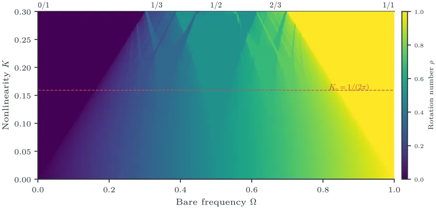
Kaneko’s first paper on nonlinear dynamics (1982) studied the period-adding phenomena in the circle map (Kaneko 1982), followed by a detailed analysis of the self-similar scaling structure (Kaneko 1983b). The question he addressed was concrete: when a single-frequency oscillator is driven by a periodic force, how does the locking structure depend on the drive amplitude? The circle map strips away all spatial extent, all amplitude dynamics, and all coupling, isolating the pure phase-locking mechanism. What Kaneko showed computationally was that the full devil’s staircase — including the complete hierarchy of period-adding sequences governed by the Farey tree — could be resolved in a single one-dimensional map. This had been analysed in parallel by Jensen, Bak, and Bohr (Jensen et al. 1983) and by Feigenbaum, Kadanoff, and Shenker (Feigenbaum et al. 1982), but Kaneko’s contribution emphasised the self-similar scaling of the period-adding sequence. We revisit Kaneko’s parameter scan from Fig. 1 of (Kaneko 1982) at finer resolution and augment it with a rotation-number staircase and Lyapunov analysis.
2.1 Circle map and Arnold tongues #
The circle map is defined by
Figure 2 shows the full tongue structure computed on a grid in the plane. Each tongue emanates from a rational at and widens as increases, with the width proportional to for small (Arnol’d 1961). The dominant tongues , , , , and are clearly visible; between them, the Farey-mediant tongues , , nest self-similarly. Below the critical line , the map is a diffeomorphism of the circle and tongues do not overlap: between any two tongues lies a gap of quasi-periodic (irrational ) motion. Above , tongues overlap, the map ceases to be invertible, and chaotic dynamics are commonly observed in the overlap regions.
How this figure was computed
# Figure: Arnold tongues -- rotation number rho(Omega, K) over a small grid.
import numpy as np

from dynachaos.maps.circle_map import rotation_number

Omega_values = np.linspace(0.0, 1.0, 10)
K_values = np.linspace(0.0, 0.3, 5)

for K in K_values:
    row = [rotation_number(K, D=Omega, n_transient=200, n_iter=1000) for Omega in Omega_values]
    locked = sum(abs(r - round(r)) < 1e-2 for r in row)
    print(f"K={K:.2f}  locked points: {locked}/{len(Omega_values)}")

# Full figure: dynachaos run sec02_circle_map
2.2 Devil’s staircase and period-adding #
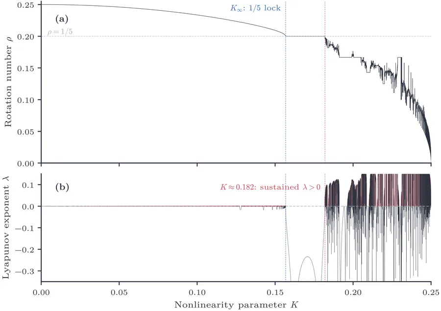
Kaneko (Kaneko 1982) studied the circle map (1) at fixed rotation frequency and swept the nonlinearity . The resulting plot of versus is a staircase-like locking curve (Figure 3): a nonincreasing function with broad rational plateaus (the frequency lockings) separated by quasi-periodic or chaotic intervals. Although the standard “complete devil’s staircase” is more often plotted as at fixed critical , Kaneko’s scan isolates the same Farey-locking mechanism along a physically important one-parameter path.
What makes the devil’s staircase “devilish”? Between any two rational plateaus and lies another plateau at the Farey mediant. This self-similar nesting continues at all scales, producing a fractal structure. At the noninvertibility threshold , mode-locked plateaus cover the full -axis; the remaining set of quasi-periodic rotation numbers is Cantor-like (Jensen et al. 1983, 1984). Below , the quasi-periodic windows have positive measure; above it, they shrink to zero. Kaneko (Kaneko 1984d) analysed the supercritical behaviour () of disordered orbits in detail. The universality of this transition was analysed independently by Feigenbaum, Kadanoff, and Shenker (Feigenbaum et al. 1982) and by Rand et al.(Rand et al. 1982; Ostlund et al. 1983).
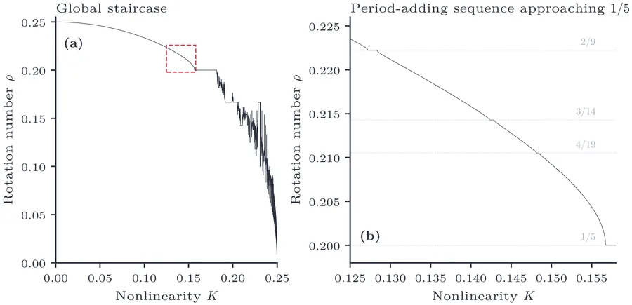
For the specific scan at , the dominant accumulation is the locking. Kaneko found that as increases toward (Feigenbaum et al. 1982), the staircase passes through the sequence , , , , with general term , before the plateau opens fully (Kaneko 1982, 1983b). Between successive members of this sequence lie narrower Farey-descendant windows, so the local structure still reflects the standard devil’s-staircase hierarchy.
2.3 Diagnostic spotlight: rotation number and Lyapunov exponent #
Figure 3 shows the staircase computed with parameter values (compared to Kaneko’s ), together with the Lyapunov exponent in a separate diagnostic panel. The rotation-number plot isolates the period-adding sequence approaching the locking, while the Lyapunov panel separates the invertible quasi-periodic regime (), the stable locked windows (), and the chaotic regime that appears after the orbit loses stability.
The Lyapunov exponent is the natural diagnostic for the circle map: it directly distinguishes locked motion () from quasi-periodic motion () and chaos (), providing a one-number summary of the dynamics at each parameter value.
How this figure was computed
# Figure: devil's staircase -- rotation number rho(A) of the circle map.
import numpy as np

from dynachaos.maps.circle_map import rotation_number

D = 0.25
A_values = np.linspace(0.0, 1.0, 20)
rho = [rotation_number(A, D=D, n_transient=500, n_iter=2000) for A in A_values]

for A, r in zip(A_values[::4], rho[::4], strict=False):
    print(f"A={A:.2f}  rho={r:.4f}")

# Full figure: dynachaos run sec02_circle_map
The self-similar locking hierarchy becomes clearer when the staircase is resolved near the onset of the plateau. Figure 4 zooms into the region containing the dominant period-adding sequence , computed with parameter values. At this scale the successive rational plateaus converging on are cleanly separated, and narrower subwindows appear between them according to the Farey-tree construction. The point of the zoom is therefore not a generic “between and ” staircase, but the specific accumulation sequence Kaneko analysed in the problem (Kaneko 1982, 1983b).
How this figure was computed
# Figure: staircase zoom -- fine A-sweep near a mode-locked plateau, with
# the Lyapunov exponent confirming the orbit is periodic (lambda < 0) there.
import numpy as np

from dynachaos.maps.circle_map import lyapunov_exponent, rotation_number

D = 0.25
A_values = np.linspace(0.15, 0.25, 10)
for A in A_values:
    rho = rotation_number(A, D=D, n_transient=500, n_iter=2000)
    lam = lyapunov_exponent(A, D=D, n_transient=500, n_iter=2000)
    print(f"A={A:.3f}  rho={rho:.4f}  lambda={lam:+.4f}")

# Full figure: dynachaos run sec02_circle_map
3 Amplitude Instability: Oscillation, Doubling, and Fractalization #
In 1984, Kaneko published “Oscillation and Doubling of Torus” (Kaneko 1984c), identifying torus oscillation as a route to chaos distinct from both frequency locking and period doubling. The phenomenon demanded a model that could support a smooth invariant circle while allowing its amplitude to destabilise independently of its phase. The delayed logistic map was Kaneko’s answer: by replacing explicit time dependence with a memory coupling (), the map preserves torus dynamics in a two-dimensional state space while permitting continuous deformation of the torus shape. What was new was the classification of three distinct fates (oscillation, doubling, and fractalization) in a single model by sweeping a single parameter ; all three are treated comprehensively in Kaneko’s monograph (Kaneko 1986a). We reproduce Kaneko’s Fig. 1 of (Kaneko 1984c) at finer parameter resolution and overlay modern diagnostics.
3.1 The delayed logistic map (canonical model) #
Kaneko (Kaneko 1984c) studied torus instabilities in their purest form using the two-dimensional delayed logistic map:
3.2 Torus oscillation #
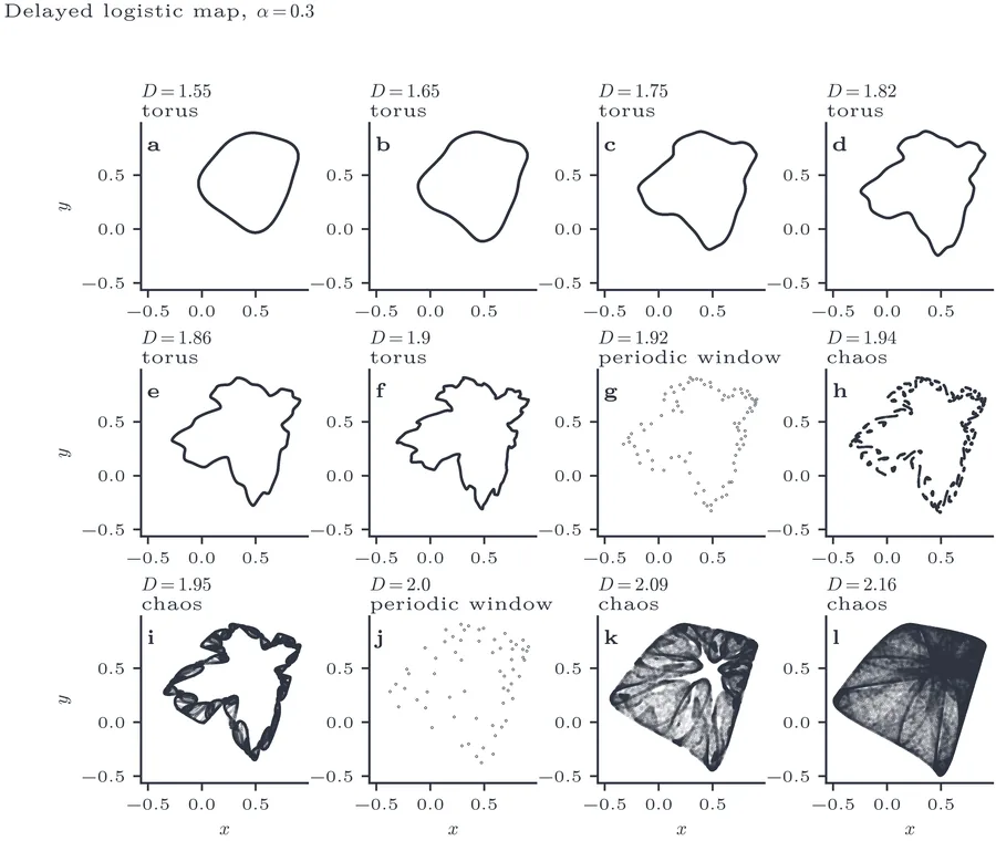
As increases beyond , the torus initially grows smoothly. But at a critical value of , the torus begins to oscillate: it develops “sidebands” in its power spectrum, corresponding to a modulation of the quasi-periodic motion. This torus oscillation was a new phenomenon, distinct from both frequency locking and torus doubling.
Kaneko classified the progression as increases at :
Smooth torus.
Torus beginning to oscillate (sidebands visible).
Frequency locking (periodic orbit inside the torus).
Chaos through torus fractalization.
Developed chaotic attractor.
The Lyapunov spectrum (Figure 7) confirms this progression quantitatively: in the torus regime and in the chaotic regime.
How this figure was computed
# Figure: attractor portraits of the delayed logistic map at A=0.3, spanning
# torus, periodic window, and chaotic D.
from dynachaos.maps.delayed_logistic import compute_attractor

A = 0.3
for D, label in ((1.55, "torus"), (1.94, "periodic window"), (2.16, "chaos")):
    traj = compute_attractor(A, D, n_transient=3000, n_plot=2000)
    print(f"D={D:.2f} ({label})  y range=[{traj[:, 1].min():.3f}, {traj[:, 1].max():.3f}]")

# Full figure: dynachaos run sec05_oscillation
The transition from locking to chaos in panels (f)–(h) of Figure 5 compresses a rich micro-structure into three frames. Figure 6 zooms into with eight closely-spaced values, each plotted with iterates. The sequence makes clear that the transition is not a single bifurcation but a compressed interval containing near-locking, relocking, and only then the loss of smooth invariant curves. Beyond , the attractor develops fractal filaments before settling into a fully chaotic cloud at the far end of the window.
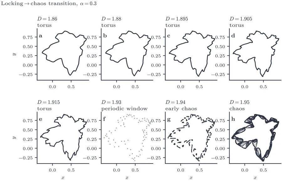
How this figure was computed
# Figure: attractors across the locking-to-chaos transition, D in [1.86, 1.95];
# lambda_1 turns positive as the frequency-locked torus gives way to chaos.
import numpy as np

from dynachaos.diagnostics.lyapunov import lyapunov_spectrum
from dynachaos.maps.delayed_logistic import delayed_logistic, delayed_logistic_jac

A = 0.3
for D in (1.860, 1.930, 1.950):
    fp = (np.sqrt(1.0 + 4.0 * D) - 1.0) / (2.0 * D)
    x0 = np.array([fp + 0.01, fp - 0.01])

    def f(state, D=D):
        return delayed_logistic(state, A, D)

    def jac(state, D=D):
        return delayed_logistic_jac(state, A, D)

    spectrum = lyapunov_spectrum(f, jac, x0, n_iter=4000, n_transient=2000)
    print(f"D={D:.3f}  lambda_1={spectrum[0]:+.4f}")

# Full figure: dynachaos run sec05_oscillation
![Lyapunov spectrum (λ1,λ2) of the delayed logistic map at α=0.3 versus D. The vertical dashed line marks the Neimark–Sacker bifurcation Dc=(3−2α)/[4(1−α)2]≈1.225.](thumbs/sec05_oscillation/lyapunov_vs_D.webp)
How this figure was computed
# Figure: Lyapunov spectrum of the delayed logistic map vs D, crossing zero
# near the torus-to-chaos transition.
import numpy as np

from dynachaos.diagnostics.lyapunov import lyapunov_spectrum
from dynachaos.maps.delayed_logistic import delayed_logistic, delayed_logistic_jac

A = 0.3
for D in (1.6, 1.95, 2.2):
    fp = (np.sqrt(1.0 + 4.0 * D) - 1.0) / (2.0 * D)
    x0 = np.array([fp + 0.01, fp - 0.01])

    def f(state, D=D):
        return delayed_logistic(state, A, D)

    def jac(state, D=D):
        return delayed_logistic_jac(state, A, D)

    spectrum = lyapunov_spectrum(f, jac, x0, n_iter=4000, n_transient=2000)
    print(f"D={D:.2f}  lambda_1={spectrum[0]:+.4f}  lambda_2={spectrum[1]:+.4f}")

# Full figure: dynachaos run sec05_oscillation
3.3 Torus doubling (Maps I and IV) #
Period doubling — the cascade that Feigenbaum showed to be universal — is the best-known route to chaos in one-dimensional maps. Kaneko (Kaneko 1983a) asked: can a torus undergo an analogous doubling?
The answer is yes. Just as a fixed point can bifurcate into a period-2 orbit (two alternating points), a smooth invariant circle ( in the map; “torus” in Kaneko’s flow language) can bifurcate into a doubled torus — a structure where the trajectory alternates between two closed curves on successive iterates. A further doubling produces a -torus, then an -torus, and so on until the tori become so convoluted that they merge into a chaotic attractor.
Kaneko studied four maps exhibiting torus doubling (Kaneko 1983a). Maps (II) and (III) are intermediate cases that interpolate between the three-dimensional Map (I) and the four-dimensional Map (IV); we focus on the two extremes. Map (I) is a three-dimensional delayed logistic:
The parameter controls how strongly the delayed variable drives the system. As increases at fixed , the torus undergoes successive doublings: , accumulating at a critical value beyond which the motion is chaotic.
Kaneko found that the doubling cascade obeys a scaling relation analogous to Feigenbaum’s:
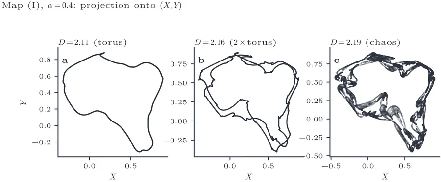
How this figure was computed
# Figure: (X, Y) projections of Map (I), the 3D delayed logistic map, across
# torus, doubled-torus, and chaotic D.
import numpy as np

from dynachaos.maps.torus_doubling import iterate_map, map_I

A = 0.4
x0 = np.array([0.5, 0.5, 0.5])
for D, label in ((2.11, "torus"), (2.16, "2x torus"), (2.19, "chaos")):
    traj = iterate_map(map_I, x0, A, D, n_transient=3000, n_plot=2000)
    print(f"D={D:.2f} ({label})  X range=[{traj[:, 0].min():.3f}, {traj[:, 0].max():.3f}]")

# Full figure: dynachaos run sec04_doubling
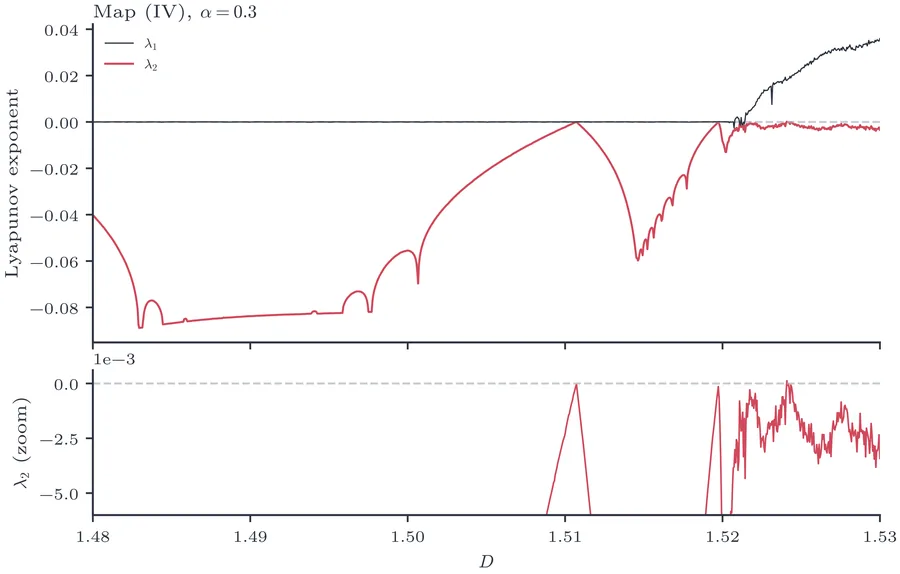
How this figure was computed
# Figure: Lyapunov spectrum of Map (IV), the 4D delayed logistic map, vs D.
import numpy as np

from dynachaos.diagnostics.lyapunov import lyapunov_spectrum
from dynachaos.maps.torus_doubling import map_IV, map_IV_jac

A = 0.3
x0 = np.array([0.5, 0.45, 0.52, 0.48])
for D in (1.50, 1.5206, 1.5212):

    def f(state, D=D):
        return map_IV(state, A, D)

    def jac(state, D=D):
        return map_IV_jac(state, A, D)

    spectrum = lyapunov_spectrum(f, jac, x0, n_iter=3000, n_transient=2000)
    print(f"D={D}  lambda_1={spectrum[0]:+.4f}  lambda_2={spectrum[1]:+.4f}")

# Full figure: dynachaos run sec04_doubling
3.4 Fractalization of torus #
What happens at the boundary between quasi-periodic motion (torus) and chaos? Kaneko (Kaneko 1984b) showed that the torus does not simply “break” into chaos; instead, it undergoes a continuous process of fractalization.
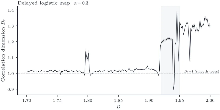
On a smooth torus, the attractor is a one-dimensional curve (a closed orbit in the Poincaré section). Its fractal dimension is exactly 1. As the control parameter approaches the chaos threshold, the curve develops wrinkles — fine-scale oscillations that fold the surface at ever smaller length scales. The fractal dimension increases continuously from 1 toward – at the onset of chaos.
This intermediate object — a geometrically fractal invariant set with nonpositive maximal Lyapunov exponent — shares the defining features of a strange nonchaotic attractor (SNA) as formalised in (Grebogi et al. 1984). (Mechanistically, classic SNAs arise in quasiperiodically forced systems; the label “SNA-like” is meant only in the geometric/dynamical sense: fractal geometry with no positive Lyapunov exponent. The qualifier is important because the delayed logistic map in this section is an autonomous two-dimensional map, not the quasiperiodically forced construction in which the classical SNA definition was introduced.)
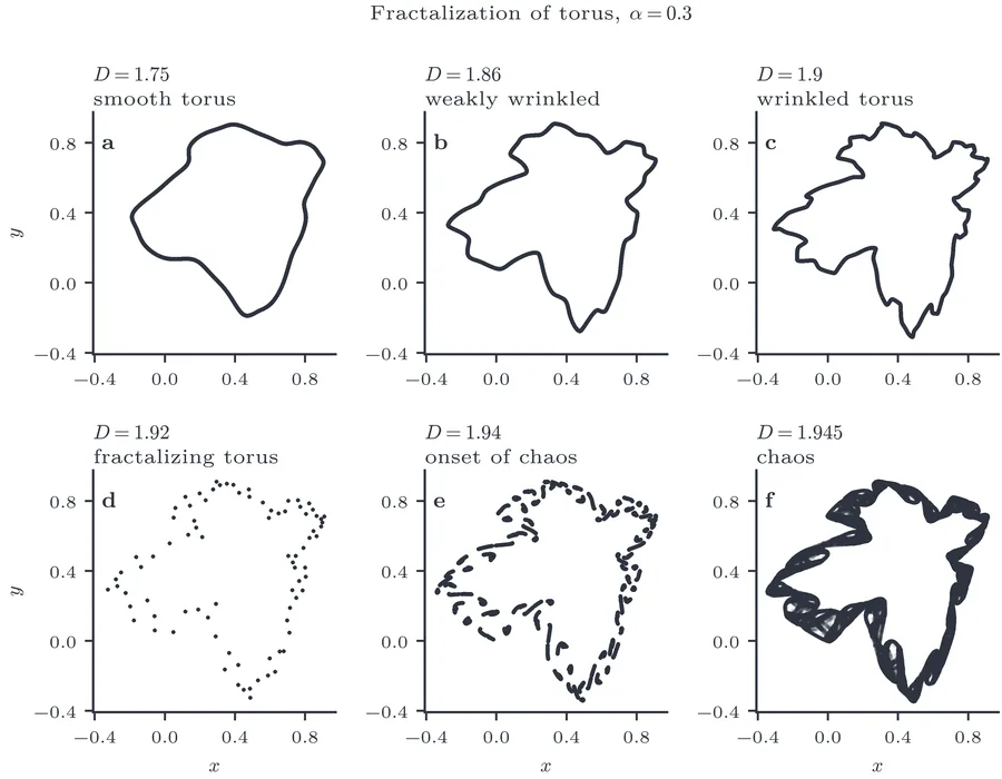
How this figure was computed
# Figure: attractor portraits of the delayed logistic map showing progressive
# fractalization of the torus as D increases from smooth to chaos onset.
from dynachaos.maps.fractalization import iterate

A = 0.3
for D, label in ((1.75, "smooth torus"), (1.92, "fractal torus"), (1.945, "chaos")):
    traj = iterate(A, D, n_transient=2000, n_record=2000)
    x_lo, x_hi = traj[:, 0].min(), traj[:, 0].max()
    print(f"D={D} ({label})  points={traj.shape[0]}  x range=[{x_lo:.3f}, {x_hi:.3f}]")

# Full figure: dynachaos run sec07_fractalization
3.5 Diagnostic spotlight: correlation dimension and SALI #
We quantify the fractalization using the Grassberger–Procaccia correlation dimension (Grassberger and Procaccia 1983). The correlation integral
Figure 11 plots versus , confirming the growth from in the smooth-torus regime to once the attractor has clearly lost smoothness. Finite-sample fluctuations and imperfect scaling-window selection produce visible non-monotone dips near the transition, so the curve should be read as a diagnostic trend rather than a strict order parameter.
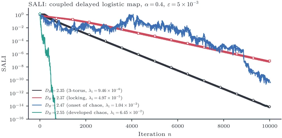
The SALI (Smaller Alignment Index) (Skokos 2001) provides a complementary alignment diagnostic. It tracks two tangent vectors under the linearised dynamics: for strongly chaotic orbits, both vectors align with the most unstable direction, so exponentially. In a two-dimensional map, however, SALI is not an ideal discriminator between invariant-circle motion and weak chaos, because the tangent space is already minimal. We therefore illustrate SALI on the four-dimensional coupled delayed logistic map introduced later in Section 5.1, using it here as a higher-dimensional analogue of the torus-to-chaos problem.
Figure 12 shows SALI time series for four regimes of that coupled delayed system. Because the map is dissipative, the two deviation vectors ultimately align with the single leading direction and SALI decays toward zero in every regime; the decay rate therefore does not cleanly separate regular from chaotic motion here, in contrast to the conservative setting for which the index was originally devised (Skokos 2001).
How this figure was computed
# Figure: correlation dimension D_2(D) rising from 1 (smooth torus) toward
# ~1.3-1.5 as the delayed logistic map approaches chaos onset.
from dynachaos.diagnostics.correlation import correlation_dimension
from dynachaos.maps.fractalization import iterate

A = 0.3
for D in (1.75, 1.90, 1.945):
    traj = iterate(A, D, n_transient=2000, n_record=3000)
    D2, _, _, _, _ = correlation_dimension(traj, n_r=30, max_pairs=200_000)
    print(f"D={D}  D2={D2:.3f}")

# Full figure: dynachaos run sec07_fractalization
How this figure was computed
# Figure: SALI decay distinguishes torus (regular) from chaotic regimes.
import numpy as np

from dynachaos.diagnostics.sali_gali import sali
from dynachaos.maps.coupled_delayed import coupled_delayed, coupled_delayed_jac

A, eps = 0.4, 5e-3
x0 = np.array([0.5, 0.5, 0.3, 0.3])

for DB, label in ((2.35, "3-torus"), (2.55, "developed chaos")):
    DA = DB + 0.1

    def f(s, DA=DA, DB=DB):
        return coupled_delayed(s, A, DA, DB, eps)

    def jac(s, DA=DA, DB=DB):
        return coupled_delayed_jac(s, A, DA, DB, eps)

    s = sali(f, jac, x0, n_iter=1000, n_transient=500)
    print(f"DB={DB} ({label})  SALI[-1]={s[-1]:.3e}")

# Full figure: dynachaos run sec11_diagnostics
4 Symmetry Breaking: Torus Collapse via Coupling #
In the same year as his torus doubling paper, Kaneko studied a different route to chaos: the transition from torus to chaos accompanied by frequency lockings with symmetry breaking(Kaneko 1983c). The question was: what happens when two identical chaotic maps are coupled symmetrically? The coupled logistic map was chosen because it is the simplest system exhibiting two-frequency quasi-periodicity from the coupling of identical subsystems, with the exchange symmetry providing a natural order parameter. What Kaneko discovered was that symmetry breaking and basin fractality arise dynamically — not from parameter-space bifurcation alone but from the topology of coexisting attractors. Takesue and Kaneko (Takesue and Kaneko 1984) subsequently showed that the resulting basin boundaries are self-similar fractals. Here we combine a coarse survey with a fixed- attractor sequence, rather than claiming a one-to-one reproduction of Kaneko’s rough fixed- regime diagram, and apply the 0-1 test as a model-free chaos diagnostic.
4.1 The coupled logistic map (canonical model) #
To study two-frequency quasi-periodicity (an invariant circle in this 2D return map), Kaneko introduced the coupled logistic map(Kaneko 1983c):
4.2 Phase diagram and symmetry-broken attractors #
Kaneko showed that as increases at fixed , the attractor can pass through a sequence of symmetry-preserving and symmetry-broken regimes:
Symmetric regular dynamics: fixed or periodic orbits with .
Locked windows: regular periodic windows embedded in the quasiperiodic route.
Symmetry breaking: the symmetry breaks, creating two coexisting attractors related by exchange.
Chaotic bands: irregular sets with positive finite-time expansion rate.
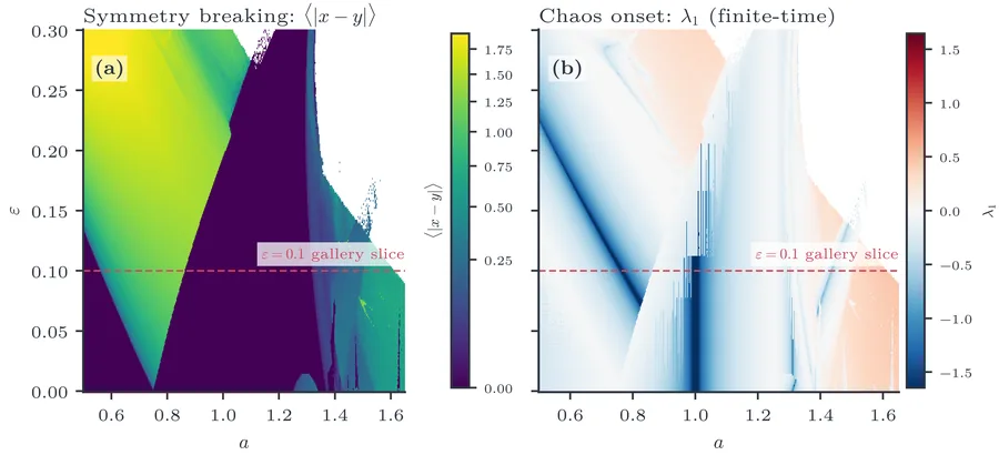
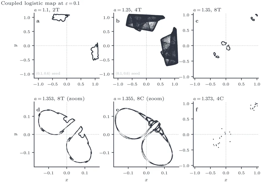
Figure 13 therefore serves as a locator map: panel (a) uses the symmetry order parameter , while panel (b) uses a finite-time estimate of the largest Lyapunov exponent . The two fields separate regions where the dynamics remains close to the invariant diagonal from regions where symmetry is broken and the motion becomes irregular. The dashed line at marks the slice used in Figure 14. That attractor gallery follows a representative branch through the route ; for the first two panels we deliberately start off the diagonal to expose the coexisting symmetry-broken tori rather than the synchronized cycles.
How this figure was computed
# Figure: symmetry breaking <|x-y|> and finite-time Lyapunov exponent lambda_1
# over a small (a, eps) grid for the coupled logistic map.
import numpy as np

from dynachaos.maps.coupled_logistic import coupled_logistic

D = 0.1
for A in (1.0, 1.2, 1.35, 1.5):
    state = np.array([0.1, 0.2])
    for _ in range(5000):
        state = coupled_logistic(state, A, D)
    asym = 0.0
    for _ in range(2000):
        state = coupled_logistic(state, A, D)
        asym += abs(state[0] - state[1])
    asym /= 2000
    print(f"a={A:.2f}  <|x-y|>={asym:.4f}")

# Full figure: dynachaos run sec03_transition
How this figure was computed
# Figure: representative attractor portraits at eps=0.1 along the
# broken-symmetry route (2T -> 4T -> 8T -> 4C).
import numpy as np

from dynachaos.maps._iter import trajectory_after_transient
from dynachaos.maps.coupled_logistic import coupled_logistic

D = 0.1
for A, label in ((1.10, "2T"), (1.25, "4T"), (1.373, "4C")):
    traj = trajectory_after_transient(
        np.array([0.1, 0.6]),
        lambda state, A=A: coupled_logistic(state, A, D),
        n_transient=5000,
        n_record=2000,
    )
    print(f"a={A:.4f} ({label})  x range=[{traj[:, 0].min():.3f}, {traj[:, 0].max():.3f}]")

# Full figure: dynachaos run sec03_transition
4.3 Self-similar basin structure #
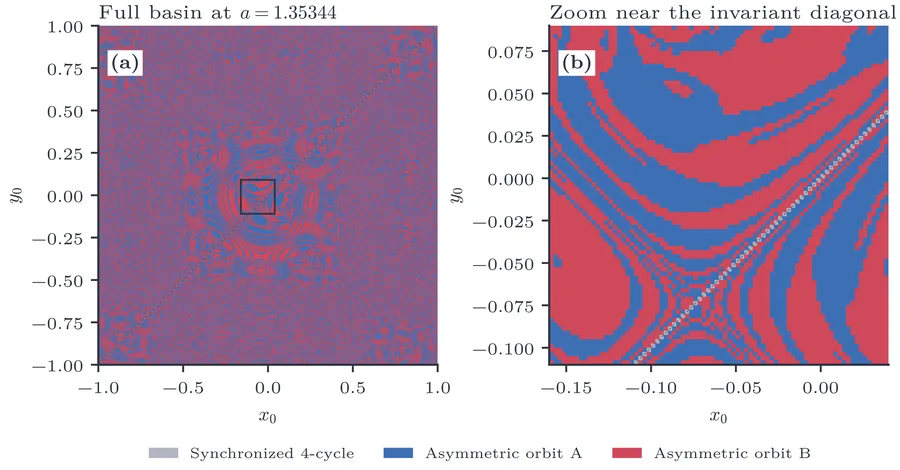
Takesue and Kaneko (Takesue and Kaneko 1984) showed that the basins of attraction for the two symmetry-broken attractors display a self-similar stripe structure: the boundary between basins is a fractal, with stripes of alternating colour at every magnification. Figure 15 reproduces this structure at on an grid. At this parameter the map has two coexisting asymmetric 4-cycles in Kaneko’s reduced notation (period-32 cycles for the original map) together with the invariant diagonal , which flows to the synchronized cycle. The zoom panel shows how the alternating blue/red stripes accumulate against that diagonal.
How this figure was computed
# Figure: basin of attraction for two mirror-image asymmetric period-32
# orbits, classified by the sign of (x-y) reached from each initial state.
# Illustrative of the method; the full figure uses
# dynachaos.maps.coupled_logistic.compute_basins, which classifies against
# two reference orbits found from a 500,000-iterate transient.
import numpy as np

from dynachaos.maps.coupled_logistic import coupled_logistic

A, D = 1.35344, 0.1
for x0 in np.linspace(-0.05, 0.05, 9):
    state = np.array([x0, -x0])
    for _ in range(20_000):
        state = coupled_logistic(state, A, D)
    basin = "A" if state[0] > state[1] else "B"
    print(f"x0={x0:+.3f}  basin={basin}  (x-y)={state[0] - state[1]:+.4f}")

# Full figure: dynachaos run sec03_transition
4.4 Diagnostic spotlight: the 0-1 test for chaos #
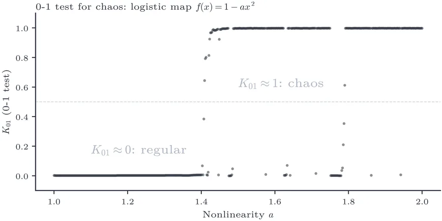
The 0-1 test (Gottwald and Melbourne 2004, 2009) provides a binary answer from a scalar time series alone: the test statistic approaches 0 for regular dynamics and 1 for chaotic dynamics. The method projects the time series onto a 2D extension via
Figure 16 shows versus for the logistic map . The periodic windows (where ) are sharply delineated from the chaotic bands (where ), reproducing the Lyapunov exponent diagram but without requiring any knowledge of the map’s equations or derivatives. That property suits the coupled logistic transition: symmetry breaking there produces complicated attractors whose Jacobian may not be readily available, leaving scalar output as the reliable input.
How this figure was computed
# Figure: 0-1 test statistic K(a) across the logistic map's route to chaos.
import numpy as np

from dynachaos.diagnostics.zero_one_test import zero_one_statistic
from dynachaos.maps.primitives import logistic

for a in (1.2, 1.6, 1.9, 2.0):
    x = 0.1
    for _ in range(2000):
        x = logistic(x, a)
    series = np.empty(2000)
    for i in range(2000):
        x = logistic(x, a)
        series[i] = x
    K = zero_one_statistic(series, n_c=20)
    print(f"a={a:.2f}  K_01={K:.3f}")

# Full figure: dynachaos run sec11_diagnostics
5 High-Dimensional Extension: Three-Torus and Forced Phase Maps #
In “Fates of Three-Torus” (Kaneko 1984a), Kaneko confronted directly the Ruelle–Takens conjecture that three-frequency quasi-periodicity should be structurally unstable. While Ruelle and Takens (Ruelle and Takens 1971) had argued that is generically destroyed by perturbations, and Grebogi, Ott, and Yorke (Grebogi et al. 1983) provided numerical evidence that three-frequency orbits are rare, Kaneko asked the more refined question: what are the possible fates? By constructing a four-dimensional coupled delayed logistic map, he stripped away all continuous-time complications and isolated the competition among three frequencies in the simplest possible discrete setting. The answer was a double devil’s staircase of lockings, a new fractalization phenomenon, and — crucially — the observation that chaos is never reached directly from but only through intermediate lockings ( cycle chaos) — a far richer catalogue than the binary “stable or unstable” verdict of Ruelle–Takens. Grebogi et al.(Grebogi et al. 1985) independently studied attractors on -tori. We reproduce the double staircase and representative projections at modern resolution.
The mechanisms in Sections 2–4 operate in one or two dimensions. What happens when a third incommensurate frequency is introduced?
5.1 The coupled delayed logistic map #
A three-torus is a quasi-periodic attractor with three independent, incommensurate frequencies . It is the dynamical object that appears in Landau’s route to turbulence (Landau 1944) after three Hopf bifurcations. Ruelle and Takens (Ruelle and Takens 1971) argued that should be structurally unstable — that generic perturbations destroy it and replace it with a strange attractor. Newhouse et al.(Newhouse et al. 1978) proved that this is indeed the case for certain perturbations. But Kaneko asked a more nuanced question: what are the possible fates of ?
To study , Kaneko constructed a four-dimensional map (Kaneko 1984a):
5.2 Lyapunov counting for -tori in maps versus flows #
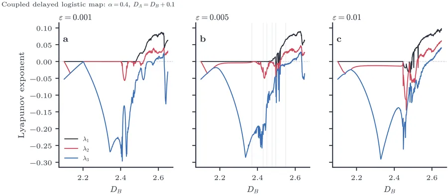
The four-dimensional Lyapunov spectrum distinguishes the dynamical regimes:
Two zero exponents, : three-frequency quasi-periodicity (a invariant set in the map, corresponding to three-torus motion in the underlying flow).
One zero exponent: two frequencies have locked; the remaining quasi-periodic motion lives on an invariant circle.
All exponents negative: fully locked periodic orbit.
: chaos (the torus has collapsed).
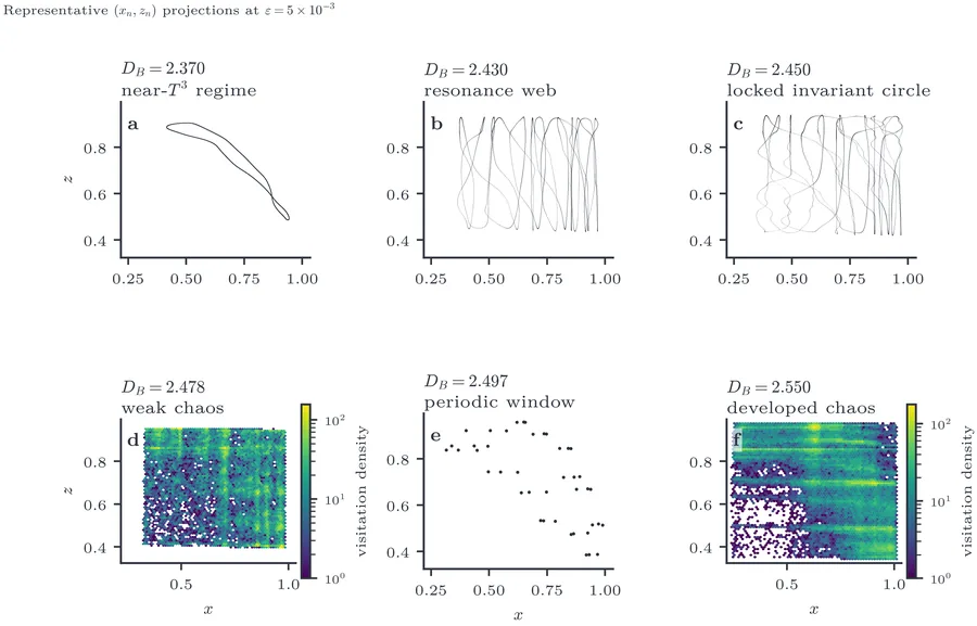
Figure 17 shows the Lyapunov spectrum versus for three values of the coupling . The corresponding projections (Figure 18) provide a geometric gallery at : a near-three-frequency curve, resonance webs and locked circles, weak chaos, a narrow periodic window, and developed chaos.
5.3 Double devil’s staircase #
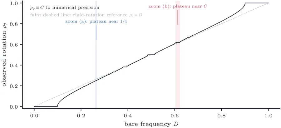
A striking prediction of Kaneko was the double devil’s staircase: when the partially locks, the rotation number takes values of the form (with and coprime), where is the irrational modulation frequency. The staircase is “double” because its plateaus are built from two basis elements ( and ), in contrast to the single-generator structure of the ordinary devil’s staircase (Kaneko 1984a). Our sweep computes the rotation numbers directly, so the staircase should be read as consistent with this two-generator locking picture rather than as an explicit rational decomposition of every plateau.
5.4 Modulated circle map #
To demonstrate the double staircase cleanly, Kaneko introduced the modulated circle map(Kaneko 1984a):
How this figure was computed
# Figure: Lyapunov spectrum of the 4D coupled delayed logistic map vs D_B,
# at fixed coupling eps, crossing from 3-torus into developed chaos.
import numpy as np

from dynachaos.diagnostics.lyapunov import lyapunov_spectrum
from dynachaos.maps.coupled_delayed import coupled_delayed, coupled_delayed_jac

A, eps = 0.4, 5e-3
x0 = np.array([0.5, 0.5, 0.3, 0.3])
for DB in (2.37, 2.478, 2.55):
    DA = DB + 0.1

    def f(state, DA=DA, DB=DB):
        return coupled_delayed(state, A, DA, DB, eps)

    def jac(state, DA=DA, DB=DB):
        return coupled_delayed_jac(state, A, DA, DB, eps)

    spectrum = lyapunov_spectrum(f, jac, x0, n_iter=2000, n_transient=1000)
    print(f"D_B={DB:.3f}  lambda_1={spectrum[0]:+.4f}  lambda_2={spectrum[1]:+.4f}")

# Full figure: dynachaos run sec06_three_torus
How this figure was computed
# Figure: (x_n, z_n) projections of the 4D coupled delayed logistic map,
# from near-T^3 quasiperiodicity through a resonance web to developed chaos.
# Illustrative of the method; the full figure uses
# dynachaos.maps.coupled_delayed.compute_projections, which samples 50,000
# points after a 30,000-iterate transient for six D_B cases.
import numpy as np

from dynachaos.maps._iter import trajectory_after_transient
from dynachaos.maps.coupled_delayed import coupled_delayed

A, eps = 0.4, 5e-3
for DB, label in ((2.37, "near-T^3"), (2.55, "developed chaos")):
    DA = DB + 0.1
    traj = trajectory_after_transient(
        np.array([0.5, 0.5, 0.3, 0.3]),
        lambda state, DA=DA, DB=DB: coupled_delayed(state, A, DA, DB, eps),
        n_transient=2000,
        n_record=1000,
        project_fn=lambda state: state[[0, 2]],
    )
    print(f"D_B={DB} ({label})  x range=[{traj[:, 0].min():.3f}, {traj[:, 0].max():.3f}]")

# Full figure: dynachaos run sec06_three_torus
How this figure was computed
# Figure: double devil's staircase -- rotation number rho_theta(D) of the
# modulated circle map, with rho_phi locked to the golden-mean frequency C.
import numpy as np

from dynachaos.maps.modulated_circle import C_GOLDEN, rotation_numbers

A, eps = 0.10, 0.05
for D in np.linspace(0.0, 1.0, 6):
    rho_theta, rho_phi = rotation_numbers(A, C_GOLDEN, D, eps, n_transient=500, n_iter=2000)
    print(f"D={D:.2f}  rho_theta={rho_theta:.4f}  rho_phi={rho_phi:.4f}")

# Full figure: dynachaos run sec06_three_torus
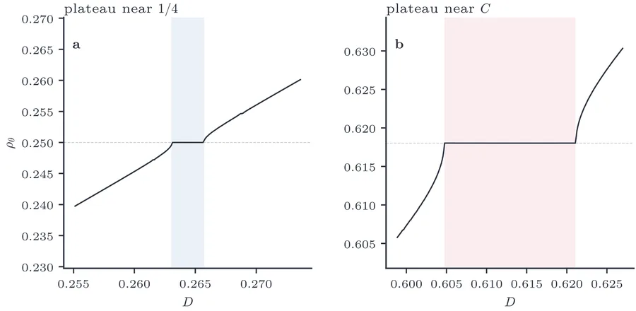
The partial locking structure becomes clearer when zoomed into narrower windows of . Figure 20 shows two such windows. Panel (a) resolves a narrow plateau near ; panel (b) shows a broader plateau near . Together they illustrate that the staircase contains both ordinary rational lockings and plateaus tied to the irrational modulation frequency.
How this figure was computed
# Figure: zoom into a mode-locked plateau of the double devil's staircase,
# where rho_theta is pinned at the rational value 1/4 across a narrow
# window of the bare frequency D (window located via the module's
# longest_plateau_window helper on the full sweep).
import numpy as np

from dynachaos.maps.modulated_circle import C_GOLDEN, rotation_numbers

A, eps = 0.10, 0.05
for D in np.linspace(0.2620, 0.2660, 8):
    rho_theta, _ = rotation_numbers(A, C_GOLDEN, D, eps, n_transient=2000, n_iter=8000)
    print(f"D={D:.4f}  rho_theta={rho_theta:.5f}")

# Full figure: dynachaos run sec06_three_torus
5.5 Diagnostic spotlight: permutation entropy and complexity-entropy plane #
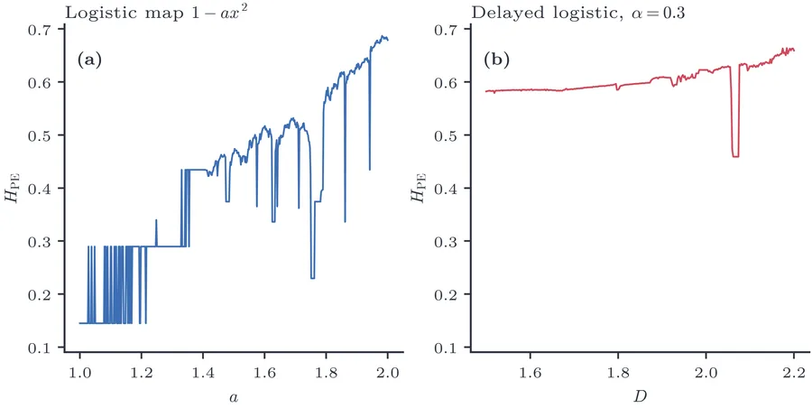
Permutation entropy (Bandt and Pompe 2002) quantifies the complexity of a time series by examining the relative ordering of consecutive values. Each window of values defines an ordinal pattern (permutation of ). The normalised Shannon entropy of the pattern distribution gives
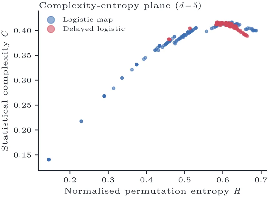
Periodic orbits produce only a few ordinal patterns (); more irregular dynamics produces many, pushing upward. Combined with the Jensen–Shannon statistical complexity (Rosso et al. 2007), the pair locates the dynamics in a complexity-entropy plane (Figure 22). Noise occupies the high-, low- corner; chaos occupies an intermediate region; and periodic motion clusters near the origin.
As a compact benchmark, we evaluate these diagnostics on scalar observables from the logistic and delayed logistic maps. This keeps the interpretation simple while showing how entropy-based diagnostics track the shift from regular to more irregular dynamics without requiring Jacobian estimates or explicit phase-space reconstructions.
How this figure was computed
# Figure: permutation entropy H_PE(a) for the logistic map.
import numpy as np

from dynachaos.diagnostics.permutation import permutation_entropy
from dynachaos.maps.primitives import logistic

for a in (1.2, 1.6, 1.9, 2.0):
    x = 0.1
    for _ in range(2000):
        x = logistic(x, a)
    series = np.empty(2000)
    for i in range(2000):
        x = logistic(x, a)
        series[i] = x
    H = permutation_entropy(series, d=5)
    print(f"a={a:.2f}  H_PE={H:.3f}")

# Full figure: dynachaos run sec11_diagnostics
How this figure was computed
# Figure: complexity-entropy plane (H, C) locating logistic-map regimes.
import numpy as np

from dynachaos.diagnostics.permutation import complexity_entropy
from dynachaos.maps.primitives import logistic

for a in (1.2, 1.6, 1.9, 2.0):
    x = 0.1
    for _ in range(2000):
        x = logistic(x, a)
    series = np.empty(2000)
    for i in range(2000):
        x = logistic(x, a)
        series[i] = x
    H, C = complexity_entropy(series, d=5)
    print(f"a={a:.2f}  H={H:.3f}  C={C:.3f}")

# Full figure: dynachaos run sec11_diagnostics
6 Spatial Extension: Coupled Map Lattices #
The coupled map lattice was Kaneko’s most influential invention (Kaneko 1985), with an earlier prelude in his study of kink-antikink dynamics (Kaneko 1984e). The CML framework was conceived as the simplest possible spatially extended dynamical system: discrete time, discrete space, continuous state. By stripping away partial-differential-equation machinery, Kaneko could study spatiotemporal chaos directly on a lattice of coupled maps. The central question was what changes when many chaotic maps are coupled together in space. The key finding was spatiotemporal intermittency (STI) — a laminar/burst coexistence whose scaling has been conjectured to belong to the directed percolation universality class (Pomeau 1986). Throughout the coupled-map-lattice and globally-coupled-map sections, “turbulent” and “turbulence” denote spatiotemporally disordered, high-dimensional chaotic phases in the coupled-map sense (Kaneko’s terminology), not solutions of the Navier–Stokes equations. Waller and Kapral (Waller and Kapral 1984) and Kapral (Kapral 1985) independently introduced similar coupled-oscillator lattice models, and Chaté and Manneville (Chaté and Manneville 1988b) later provided detailed studies of the STI transition. In what follows we reproduce Kaneko’s spacetime diagrams and a variance-based activity map at – finer resolution, and use recurrence quantification analysis as a modern single-site benchmark.
6.1 CML definition and three models #
A coupled map lattice (CML) is a discrete-time, discrete-space dynamical system (Kaneko 1985):
Kaneko studied three CML models with different local dynamics:
Piecewise linear map with .
Coupled circle maps with and .
Coupled logistic maps with and .
6.2 Spatiotemporal intermittency and directed percolation #
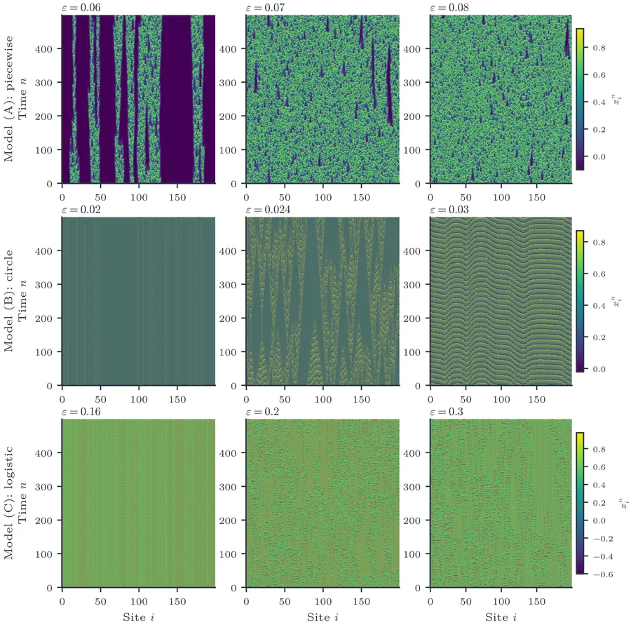
All three models exhibit spatiotemporal intermittency (STI): the spacetime diagram (Figure 23) shows alternating laminar (ordered) and burst (disordered) regions. As the coupling is tuned, the fraction of bursts changes continuously, analogous to a phase transition.
Kaneko reduced the laminar/burst dynamics to a binary (cellular automaton) description (Kaneko 1985) and characterised the transition through burst-propagation speed with –, and the growth of positive Lyapunov exponents. Pomeau (Pomeau 1986) suggested a connection to the universality class of directed percolation (DP), a fundamental paradigm in non-equilibrium statistical mechanics (Hinrichsen 2000). Chaté and Manneville (Chaté and Manneville 1988b, 1988a) investigated this connection and found DP-like scaling features in deterministic spatiotemporal intermittency, while noting that the critical exponents may depend on whether the laminar state is strictly absorbing (Chaté and Manneville 1989b, 1989a); Kaneko himself noted that “the universality class on critical exponents seems to be different” (Kaneko 1989b).
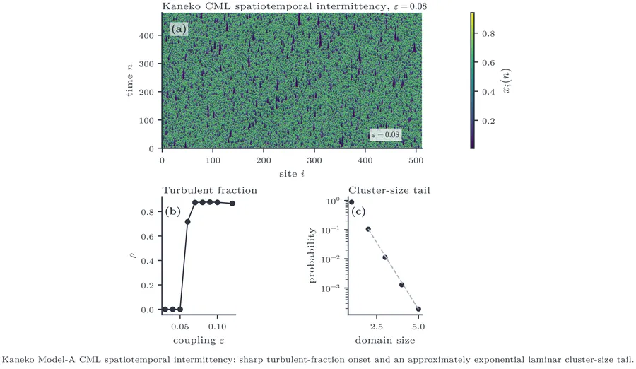
To complement the qualitative spacetime view with quantitative measures, we extract an STI “spine” from the Kaneko Model-A CML (Figure 24): the turbulent fraction as a function of the coupling , together with the laminar-domain size distribution. The turbulent fraction has a sharp onset: is near zero below and then rises steeply to a burst-dominated plateau near . The laminar cluster-size distribution shows an approximately exponential tail (decay rate over the accessible range), consistent with the DP-like phenomenology while remaining agnostic on the exact universality class, in line with the caveats above.
How this figure was computed
# Figure: spacetime diagrams of a coupled map lattice (Kaneko 1985 Model C,
# logistic local map) at three couplings spanning frozen, pattern, and
# turbulent regimes -- shown here via each snapshot's spatial variance.
from dynachaos.cml.spatiotemporal import model_C_f, simulate_cml

N = 60
for eps in (0.16, 0.20, 0.30):
    spacetime = simulate_cml(model_C_f, model_C_f, eps, N=N, n_transient=200, n_record=50)
    print(f"eps={eps:.2f}  final-row var={spacetime[-1].var():.4f}")

# Full figure: dynachaos run sec08_sti
How this figure was computed
# Figure: Kaneko Model-A CML spatiotemporal intermittency -- the turbulent
# fraction (sites with |x(i+1)-x(i)| > delta, the Kaneko 1985 burst
# criterion) rises sharply with coupling eps.
import numpy as np

from dynachaos.cml.spatiotemporal import model_A_f, simulate_cml

N = 80
rng = np.random.default_rng(42)
for eps in (0.05, 0.08, 0.12):
    x0 = rng.uniform(0, 1, N)
    spacetime = simulate_cml(model_A_f, model_A_f, eps, N=N, n_transient=300, n_record=60, x0=x0)
    turbulent_mask = np.abs(spacetime - np.roll(spacetime, -1, axis=1)) > 0.05
    print(f"eps={eps:.2f}  turbulent_fraction={turbulent_mask.mean():.3f}")

# Full figure: dynachaos run sec12_intermittency
6.3 Pattern dynamics (five phases) #
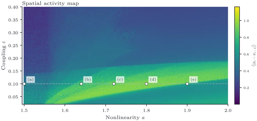
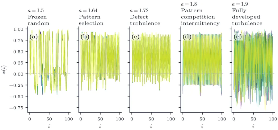
Kaneko (Kaneko 1989b) systematically classified the dynamics of the CML (13) with the logistic map and . The canonical taxonomy in the plane contains five phases:
Frozen random (, moderate ): the lattice settles into a static, spatially disordered pattern.
Pattern selection (–): the lattice spontaneously selects a spatially periodic pattern, breaking translational symmetry.
Defect turbulence (–): the selected pattern is disrupted by defects (domain walls) that nucleate, propagate, and annihilate chaotically.
Pattern competition intermittency (–): large coherent domains compete for territory, punctuated by intermittent bursts of turbulence.
Fully developed turbulence (): all spatial coherence is lost.
Figure 25 shows a variance-based activity map computed on a grid (versus Kaneko’s ). Because the plotted observable is only the temporal variance of one representative site, the figure should be read as a locator map consistent with the five-phase taxonomy, not as an automatic phase classifier. Figure 26 then shows space-amplitude plots at for five values of marked on that map.
How this figure was computed
# Figure: global phase diagram of the logistic coupled map lattice
# (Kaneko 1989); spatial activity <|x_i - x_{i-1}|> distinguishes frozen,
# pattern, and turbulent phases across (a, eps).
import numpy as np

from dynachaos.cml.primitives import cml_step_logistic as cml_step

N = 40
rng = np.random.default_rng(42)
for a, eps in ((1.50, 0.10), (1.72, 0.10), (1.90, 0.10)):
    x = rng.uniform(-1, 1, N)
    for _ in range(500):
        x = cml_step(x, a, eps)
    activity = 0.0
    for _ in range(200):
        x = cml_step(x, a, eps)
        activity += np.mean(np.abs(x - np.roll(x, 1)))
    print(f"a={a:.2f} eps={eps:.2f}  spatial activity={activity / 200:.4f}")

# Full figure: dynachaos run sec09_pattern
How this figure was computed
# Figure: space-amplitude snapshots x(i) vs site i of a logistic coupled
# map lattice, showing how spatial structure sharpens from a frozen random
# pattern toward fully developed turbulence.
import numpy as np

from dynachaos.cml.primitives import cml_step_logistic as cml_step

N = 40
rng = np.random.default_rng(42)
for a, eps, label in ((1.50, 0.10, "frozen random"), (1.90, 0.10, "fully developed turbulence")):
    x = rng.uniform(-1, 1, N)
    for _ in range(500):
        x = cml_step(x, a, eps)
    snapshot = x.copy()
    print(f"a={a:.2f} ({label})  amplitude mean={snapshot.mean():.4f} std={snapshot.std():.4f}")

# Full figure: dynachaos run sec09_pattern
6.4 Co-moving Lyapunov exponent and information flow #
Kaneko (Kaneko 1986b) introduced the co-moving Lyapunov exponent to quantify how perturbations propagate through a CML. Consider a localised perturbation evolving under the linearised CML dynamics:
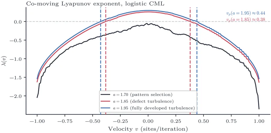
Figure 27 shows for three CML regimes: pattern selection (), defect turbulence (), and fully developed turbulence (). In the present finite-time estimate, the pattern-selection curve stays below zero for all sampled velocities, while the defect-turbulent and fully developed turbulent cases show clear zero-crossings that mark propagation speeds.
How this figure was computed
# Figure: co-moving Lyapunov exponent lambda(v) for a logistic coupled map
# lattice; its zero crossings mark the propagation velocities of chaotic
# information in the spatiotemporal state.
import numpy as np

from dynachaos.diagnostics.comoving_lyapunov import comoving_lyapunov_spectrum_logistic

v_values = np.array([-0.5, 0.0, 0.5])
for a in (1.70, 1.85, 1.95):
    lam_v = comoving_lyapunov_spectrum_logistic(
        a=a, eps=0.3, N=60, v_values=v_values, n_iter=3000, n_transient=500
    )
    print(f"a={a:.2f}  lambda(v)={np.round(lam_v, 4)}")

# Full figure: dynachaos run sec08_sti
6.5 Thermodynamics of spatiotemporal chaos #
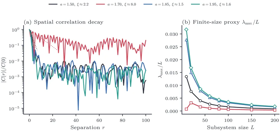
For a CML with sites, the full Lyapunov spectrum grows with system size. Kaneko (Kaneko 1989c) introduced the concept of intensive thermodynamic quantities for spatiotemporal chaos: the KS entropy density , the Lyapunov dimension density , and the density of positive Lyapunov exponents. When the spatial correlation length is much smaller than the system size , these densities converge to well-defined intensive values — the CML behaves like a thermodynamic system with local degrees of freedom.
This convergence breaks down near phase transitions (where ) and in the pattern selection phase (where long-range spatial order imposes correlations across the lattice). Figure 28 combines the spatial correlation function with a finite-size proxy, , based on the maximal Lyapunov exponent of a subsystem of size . Taken together, the curves are consistent with short, few-site correlation lengths together with slower finite-size convergence in the frozen and pattern-selection cases, but they should not be read as a rigorous thermodynamic proof on their own.
How this figure was computed
# Figure: spatial autocorrelation C(r)/C(0) of a logistic coupled map
# lattice, decaying from 1 as separation r grows -- faster decay signals a
# shorter correlation length as the nonlinearity a increases toward chaos.
import numpy as np

from dynachaos.cml.primitives import cml_step_logistic as cml_step

N = 60
eps = 0.3
rng = np.random.default_rng(42)
for a in (1.5, 1.85, 1.95):
    x = rng.uniform(-0.5, 0.5, N)
    for _ in range(500):
        x = cml_step(x, a, eps)
    snapshots = np.empty((200, N))
    for s in range(200):
        x = cml_step(x, a, eps)
        snapshots[s] = x
    fluct = snapshots - snapshots.mean()
    fft_f = np.fft.rfft(fluct, axis=1)
    power = (fft_f * np.conj(fft_f)).real
    full_corr = np.fft.irfft(power, n=N, axis=1).mean(axis=0) / N
    c_norm = full_corr / full_corr[0]
    print(f"a={a:.2f}  C(r=0..3)/C(0)={np.round(c_norm[:4], 3)}")

# Full figure: dynachaos run sec08_sti
6.6 Diagnostic spotlight: RQA and spacetime recurrence #
Recurrence plots (Eckmann et al. 1987; Marwan et al. 2007) visualise the times at which a trajectory returns to a previously visited neighbourhood. From the binary recurrence matrix (where is the recurrence threshold), one extracts quantitative measures:
RR (recurrence rate): fraction of recurrent points.
DET (determinism): fraction in diagonal lines ().
LAM (laminarity): fraction in vertical lines ().
ENTR: Shannon entropy of the diagonal line length distribution.
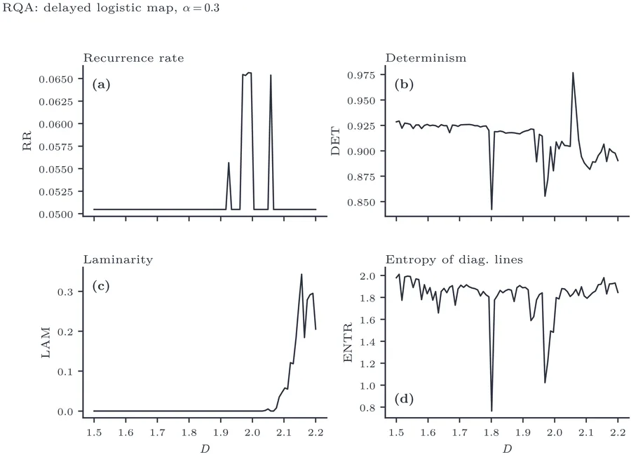
RQA is a natural diagnostic for the laminar/burst dichotomy that defines STI: the laminarity measure LAM tracks the fraction of near-recurrent (laminar) states, while ENTR captures the structural complexity of the laminar/burst boundaries.
We illustrate the four RQA measures on the delayed logistic map (Section 3.1), whose torus-to-chaos transition provides a controlled single-site benchmark before any extension to the high-dimensional CML setting, where additional embedding-dimension choices arise. Figure 29 shows these four measures versus for the delayed logistic map. The transition from torus to chaos manifests as a jump in ENTR and a restructuring of DET and LAM.
How this figure was computed
# Figure: RQA measures (RR, DET, LAM, ENTR) along the delayed logistic map.
import numpy as np

from dynachaos.diagnostics.recurrence import recurrence_matrix, rqa
from dynachaos.maps.primitives import delayed_logistic

A = 0.3
for D in (1.6, 1.9, 2.1):
    state = np.array([0.51, 0.49])
    for _ in range(2000):
        state = delayed_logistic(state, A, D)
    traj = np.empty((500, 2))
    for i in range(500):
        state = delayed_logistic(state, A, D)
        traj[i] = state
    R, _ = recurrence_matrix(traj, percentile=5)
    stats = rqa(R, l_min=2, v_min=2)
    print(f"D={D:.2f}  RR={stats['RR']:.3f}  DET={stats['DET']:.3f}  LAM={stats['LAM']:.3f}")

# Full figure: dynachaos run sec11_diagnostics
6.7 Diagnostic spotlight: the temporal-intermittency taxonomy #
The laminar/burst dichotomy that organises spatiotemporal intermittency has a classical low-dimensional counterpart. Pomeau and Manneville (Pomeau and Manneville 1980) classified the intermittent routes to chaos by the way a periodic orbit loses stability: Type I through a tangent (saddle–node) bifurcation, Type II through a subcritical Hopf bifurcation, and Type III through a subharmonic (inverse period-doubling) bifurcation. A distinct mechanism, on–off intermittency, arises when an invariant subspace loses transverse stability at a blowout bifurcation (Platt et al. 1993; Heagy et al. 1994). We apply the same laminar-phase detection and heavy-tail estimators used above (maximum-likelihood exponent with bootstrap confidence interval and a goodness-of-fit -value) to canonical realisations of each route, as a check that the diagnostics behave correctly where the underlying scaling laws are known.
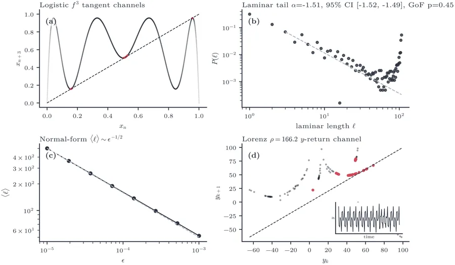
Type I (Figure 30) is realised by the logistic map just below its period-3 window, where three tangent channels open between the third iterate and the diagonal. The laminar-length distribution follows a power law (, goodness-of-fit ) and the mean laminar length obeys the normal-form scaling ; the Lorenz system at provides a continuous-time exemplar of the same near-diagonal reinjection channel.
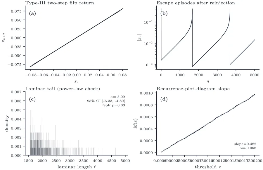
Type III (Figure 31) is illustrated through the flip channel of a second-iterate return map, with the reinjection probability density characterised in the del Río–Elaskar formulation (Río and Elaskar 2010; Elaskar et al. 2011).
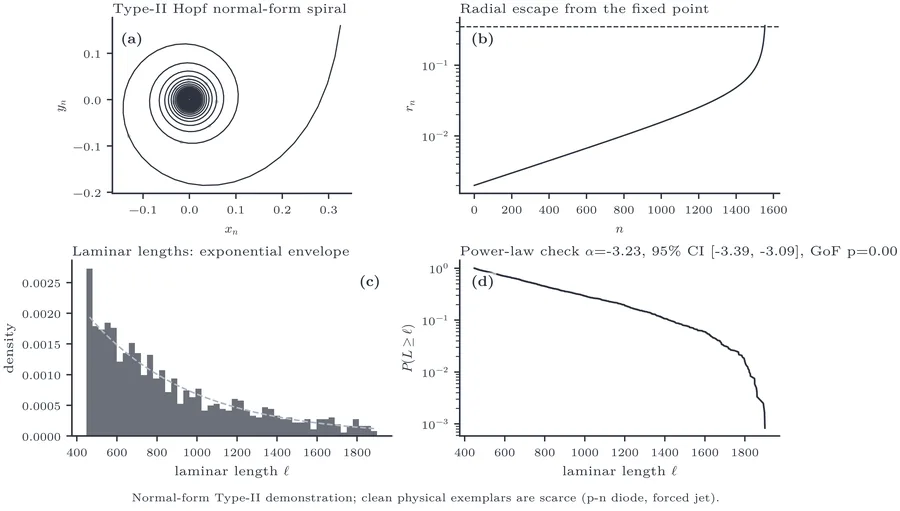
Type II (Figure 32) is shown only as a normal-form demonstration: the spiral growth and reinjection of the subcritical-Hopf normal form yield a laminar-length distribution with an exponential (not power-law) envelope, and a power-law fit is correctly rejected (goodness-of-fit ). Clean physical Type II exemplars are scarce (the p–n diode and the forced jet are the usual citations), so we make no claim beyond the normal form.
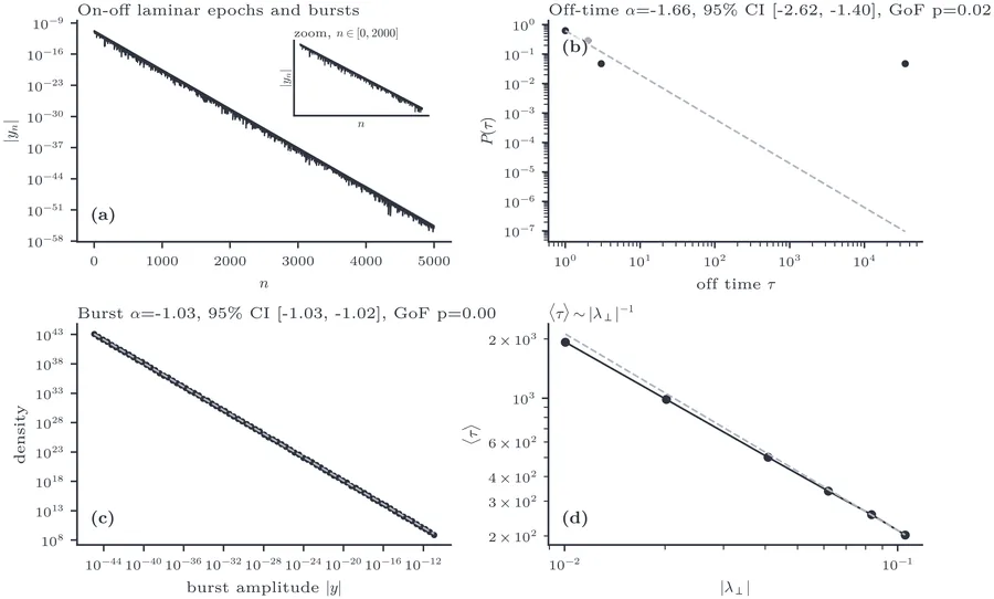
On–off intermittency (Figure 33) uses a skew logistic system tuned just past its blowout onset, where the transverse Lyapunov exponent crosses zero. The off-time (laminar) distribution is heavy-tailed with a measured exponent (95% CI ); the interval is wide and only loosely brackets the canonical value rather than confirming it. The mean off-time follows the expected scaling . The burst-amplitude distribution is an honest negative: it is not a power law (goodness-of-fit ), and we report it as such rather than forcing a fit.
Taken together, these temporal routes supply a vocabulary rather than a decomposition for the spatiotemporal case. Each laminar interval in the coupled-map-lattice intermittency of Section 6.1 is, locally in time, a site lingering near a marginally stable state before a burst, and the classical types catalogue the ways such local stability can be lost — without implying that any single type accounts for the full lattice dynamics, which couple these local events across space.
How this figure was computed
# Figure: Type-I intermittency (tangent bifurcation) -- the logistic map
# near its period-3 saddle-node onset r_c = 1+sqrt(8) produces long
# laminar phases separated by chaotic bursts; here we print their lengths.
from dynachaos.diagnostics.intermittency import detect_laminar_phases
from dynachaos.maps.intermittency import LOGISTIC_TYPE_I_ONSET, logistic_type_i_oracle

series = logistic_type_i_oracle(20_000, x0=0.2, r=LOGISTIC_TYPE_I_ONSET - 1e-4)
_, lengths = detect_laminar_phases(series, method="period", period=3, percentile=70.0)
print(
    f"r_c={LOGISTIC_TYPE_I_ONSET:.4f}  n_laminar_phases={len(lengths)}  "
    f"mean_length={lengths.mean():.2f}"
)

# Full figure: dynachaos run sec12_intermittency
How this figure was computed
# Figure: Type-III intermittency (subharmonic/flip bifurcation) -- the
# sign-alternating flip normal form x -> -(1+eps)x - a*x^3 grows slowly
# and laminar-phase length increases as the reinjection amplitude shrinks.
# Illustrative of the method; the full figure uses
# dynachaos.diagnostics.type_iii_intermittency_figure's escape-episode
# statistics, built on this same flip recurrence
# (dynachaos.maps.intermittency.pm_type_iii_oracle).
import numpy as np

from dynachaos.maps.intermittency import pm_type_iii_oracle

eps, a, escape_threshold = 2e-3, 1.0, 0.35
for x0 in (2e-6, 2e-4, 2e-3):
    orbit = pm_type_iii_oracle(8000, x0=x0, eps=eps, a=a)
    escape_idx = int(np.argmax(np.abs(orbit) >= escape_threshold))
    print(f"x0={x0:.0e}  laminar_length={escape_idx} steps before escape")

# Full figure: dynachaos run sec12_intermittency
How this figure was computed
# Figure: Type-II intermittency (subcritical Hopf) -- an unstable spiral
# with slow growth rate eps produces long near-periodic laminar episodes
# before escaping past a threshold radius; escape length grows as the
# reinjection radius shrinks. Illustrative of the method; the full figure
# uses dynachaos.diagnostics.type_ii_intermittency_figure's bounded-orbit
# escape-time computation, built on the same normal-form recurrence as
# dynachaos.maps.intermittency.pm_type_ii_oracle.
import warnings

import numpy as np

from dynachaos.maps.intermittency import pm_type_ii_oracle

eps, a, theta, escape_threshold = 2e-3, 1.0, 0.17, 0.35
with warnings.catch_warnings():
    warnings.filterwarnings("ignore", category=RuntimeWarning)
    for r0 in (1e-3, 1e-2, 2e-2):
        orbit = pm_type_ii_oracle(2500, x0=r0, y0=0.0, eps=eps, a=a, theta=theta)
        radius = np.linalg.norm(orbit, axis=1)
        escape_idx = int(np.argmax(radius >= escape_threshold))
        print(f"r0={r0:.0e}  laminar_length={escape_idx} steps before escape")

# Full figure: dynachaos run sec12_intermittency
How this figure was computed
# Figure: on-off intermittency -- a logistic-driven skew-product whose
# transverse Lyapunov exponent lambda_perp = log(2*eps) approaches zero as
# eps -> 0.5 (blowout onset); the transverse amplitude alternates between
# quiescent ("off", below the 90th percentile) and bursting phases. We
# print lambda_perp and the mean off-phase (laminar) run length observed
# in each short realization.
import numpy as np

from dynachaos.maps.intermittency import ON_OFF_SKEW_LOGISTIC_ONSET, on_off_skew_logistic_oracle


def mean_run_length(mask):
    lengths, run = [], 0
    for flag in mask:
        if flag:
            run += 1
        elif run > 0:
            lengths.append(run)
            run = 0
    if run > 0:
        lengths.append(run)
    return np.mean(lengths) if lengths else 0.0


for eps in (0.45, 0.48, ON_OFF_SKEW_LOGISTIC_ONSET - 0.01):
    skew = on_off_skew_logistic_oracle(20_000, x0=0.217, y0=1e-2, eps=eps)
    y = np.abs(skew[1000:, 1])
    off_mask = y <= np.percentile(y, 90)
    lambda_perp = np.log(2.0 * eps)
    print(
        f"eps={eps:.3f}  lambda_perp={lambda_perp:+.4f}  "
        f"mean_off_run_length={mean_run_length(off_mask):.1f}"
    )

# Full figure: dynachaos run sec12_intermittency
7 Mean-Field Extension: Globally Coupled Maps #
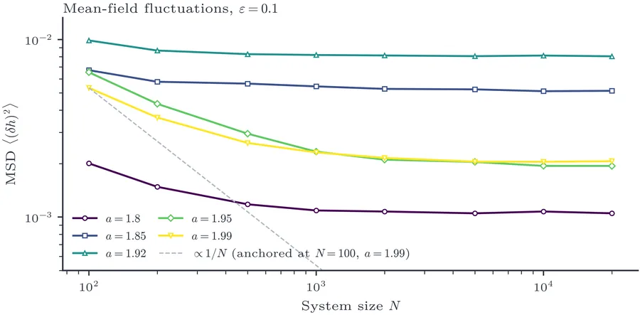
In 1989–1990, Kaneko introduced the globally coupled map (Kaneko 1990b, 1989a) and posed a question that went beyond the spatial phenomenology of CML: can a system be microscopically chaotic yet macroscopically non-self-averaging? The GCM replaces nearest-neighbour diffusion with all-to-all coupling — the mean-field limit of the CML. This deliberate simplification strips away all spatial structure, isolating the interplay between individual chaos and collective order. What Kaneko discovered was a trio of phenomena impossible in nearest-neighbour CMLs: dynamical clustering (spontaneous symmetry breaking among identical elements), violation of the law of large numbers (the mean field retains finite fluctuations as ), and collective chaos (the mean field itself has low-dimensional chaotic dynamics). The clustering phenomenon was further developed in (Kaneko 1990a, 1991, 1992a). We reproduce Kaneko’s MSD-versus- plot (Fig. 1 of (Kaneko 1990b)) and add new visualisations of cluster states and the collective Lyapunov exponent.
Kaneko (Kaneko 1990b) introduced the globally coupled map (GCM):
7.1 Violation of the law of large numbers #
Kaneko’s thesis can be stated sharply: collective chaos violates the law of large numbers but not the central limit theorem — approaches Gaussian form, yet its variance remains macroscopic (Kaneko 1990b).
For independent, identically distributed random variables, the variance of the mean decreases as — this is the law of large numbers. Kaneko showed that for the GCM at certain parameter values, the mean-square deviation (MSD)
This “violation of the law of large numbers” (more precisely, a failure of the usual scaling) is a manifestation of collective chaos(Shibata and Kaneko 1998): the mean field itself undergoes low-dimensional chaotic motion, decoupled from the high-dimensional dynamics of individual sites. With increasing , the distribution of the mean field (Figure 35) approaches an approximately Gaussian form, yet its variance stops decreasing beyond a crossover size, so the law of large numbers fails while CLT-like Gaussianity can still hold (Kaneko 1990b, 1992a).
7.2 Collective chaos and cluster states #
The nontrivial mean-field dynamics indicates that the oscillators, although not synchronised, maintain correlations that resist averaging. Kaneko showed that the system self-organises into cluster states: groups of oscillators that share the same trajectory, with the number and sizes of clusters depending on and . These clusters are not imposed by the coupling topology (which is all-to-all and thus featureless) but emerge spontaneously from the dynamics — a form of dynamical symmetry breaking.
How this figure was computed
# Figure: mean-square displacement (variance) of the mean field h_n of a
# globally coupled logistic map vs system size N; Kaneko's result is that
# this MSD decays much slower than the naive N^-1 central-limit rate (and
# saturates at large N/sample size), a law-of-large-numbers violation.
# This demo, at much smaller N and sample size than the full figure,
# already shows a 100x increase in N shrinking the variance by under 5x.
import numpy as np

from dynachaos.cml.primitives import gcm_step
from dynachaos.maps.primitives import logistic

a = 1.99
eps = 0.1
rng = np.random.default_rng(42)
for N in (50, 500, 5000):
    x = rng.uniform(-1, 1, N)
    for _ in range(300):
        x = gcm_step(x, a, eps)
    h_series = np.empty(400)
    for t in range(400):
        x = gcm_step(x, a, eps)
        h_series[t] = np.mean(logistic(x, a))
    print(f"N={N:5d}  Var(h)={np.var(h_series):.3e}")

# Full figure: dynachaos run sec10_gcm
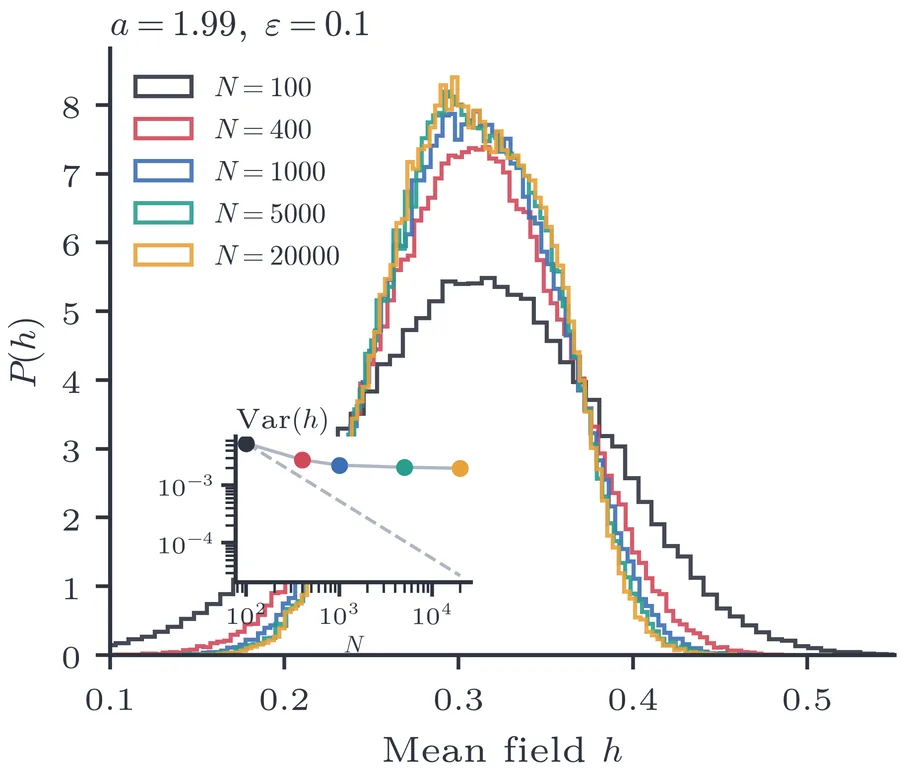
How this figure was computed
# Figure: distribution P(h) of the mean field h_n of a globally coupled
# logistic map; the mean-field histogram stays broad rather than narrowing
# to a delta function as N grows, the hallmark of GCM violating the law
# of large numbers.
import numpy as np

from dynachaos.cml.primitives import gcm_step
from dynachaos.maps.primitives import logistic

a = 1.99
eps = 0.1
rng = np.random.default_rng(42)
for N in (50, 5000):
    x = rng.uniform(-1, 1, N)
    for _ in range(300):
        x = gcm_step(x, a, eps)
    h_series = np.empty(400)
    for t in range(400):
        x = gcm_step(x, a, eps)
        h_series[t] = np.mean(logistic(x, a))
    print(f"N={N:5d}  mean(h)={h_series.mean():.4f}  std(h)={h_series.std():.4f}")

# Full figure: dynachaos run sec10_gcm
7.3 Clustered attractors and switching #
In the GCM, a cluster state is a partition of the sites into groups with nearly identical instantaneous values at a given iterate. The partition is characterised by the cluster multiplicities with . Kaneko (Kaneko 1990a) showed that at moderate coupling (), the GCM spontaneously selects a small number of clusters (–), and that the partition coding provides a discrete “label” for each macroscopic state.
A remarkable discovery was posi-nega switching(Kaneko 1989a): the system can hop between different clustered attractors under controlled perturbations that change the cluster size partition. This switching is not random noise but follows deterministic rules governed by the basin structure of the clustered attractors (Kaneko 1991). Figure 36 visualises the cluster structure as a spacetime diagram after sorting the site values at each time step, so that coherent clusters appear as broad plateaus whose widths encode their populations.
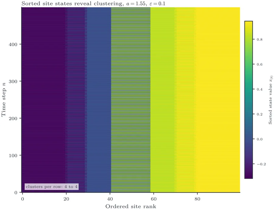
How this figure was computed
# Figure: cluster count of a globally coupled logistic map (Kaneko 1990);
# sites that converge to (near-)identical states form a coherent cluster.
from dynachaos.cml.gcm_clusters import compute_clusters

for eps in (0.1, 0.3):
    result = compute_clusters(
        a=1.55,
        eps=eps,
        n_sites=40,
        n_transient=2000,
        n_record=10,
        output_path=None,
    )
    n_clusters = len(set(result["cluster_labels"][-1]))
    print(f"eps={eps:.2f}  clusters at final step={n_clusters}")

# Full figure: dynachaos run sec10_gcm
7.4 Collective degrees of freedom #
Shibata and Kaneko (Shibata and Kaneko 1998) showed that the mean field of the GCM can have a positive collective Lyapunov exponent: a small perturbation to the macroscopic mean field grows exponentially, even though the microscopic dynamics of individual sites may be independently chaotic with very different exponents. This defines a collective chaos phase in which the macroscopic observable has its own low-dimensional chaotic dynamics, distinct from the high-dimensional microscopic chaos.
The partially ordered (PO) phase — intermediate between full synchronisation and full turbulence — is characterised by clusters that form, merge, and split in a marginally stable regime. Kaneko (Kaneko 1994a) showed that in this regime, information cascades through the cluster hierarchy with marginal stability: the system sits at the edge of a bifurcation, generating long-range temporal correlations. Takeuchi, Ginelli, and Chaté (Takeuchi et al. 2009) later showed that co-moving Lyapunov analysis in large CML systems helps quantify collective dynamics. Figure 37 plots a finite-time estimate of the collective Lyapunov exponent as a function of .
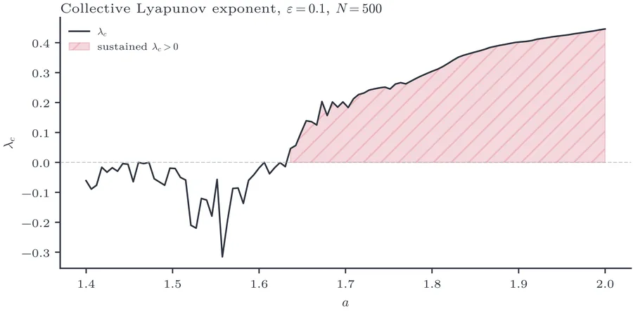
How this figure was computed
# Figure: collective Lyapunov exponent lambda_c of the mean field of a
# globally coupled logistic map (Kaneko 1990); lambda_c > 0 marks
# collective chaos of the macroscopic mean field itself.
from dynachaos.cml.gcm_clusters import compute_collective

result = compute_collective(
    eps=0.1,
    n_sites=60,
    a_values=[1.5, 1.85, 1.99],
    n_transient=200,
    n_measure=2000,
    renorm_interval=10,
    output_path=None,
    progress_interval=0,
)
for a, lam_c in zip(result["a_values"], result["lyap_c"]):
    print(f"a={a:.2f}  lambda_c={lam_c:.4f}")

# Full figure: dynachaos run sec10_gcm
7.5 Impact within the 1990s #
Kaneko’s GCM programme generated several lines of sustained investigation during the 1990s. Dynamic clustering provided a framework for understanding cell differentiation in biological networks (Kaneko 1994b, 1997a): the spontaneous partition of identical coupled elements into distinct groups mirrors the emergence of cell types from genetically identical precursors. The discovery of Milnor attractor dominance (Kaneko 1997b, 1998) — where noise-induced transitions between coexisting attractors are governed not by basin volume but by the Milnor attractor structure — opened connections to stochastic dynamics and ergodic theory. These developments transformed the GCM from a model of spatiotemporal chaos into a general framework for complex-systems dynamics.
8 Glossary #
For readers unfamiliar with nonlinear dynamics, we collect concise definitions of the key concepts appearing throughout this paper.
- Arnold tongue
A wedge-shaped region in the two-parameter plane of a periodically forced oscillator within which the oscillator frequency locks to a rational multiple of the driving frequency. Named after V. I. Arnol’d.
- Collective chaos
Chaotic dynamics of the macroscopic mean field in a system of many coupled elements, persisting even as the number of elements .
- Devil’s staircase
A monotone function (typically rotation number versus a parameter) consisting of infinitely many rational plateaus (lockings) interspersed with a Cantor set of irrational values.
- Directed percolation (DP)
A non-equilibrium phase transition universality class describing the spreading of an “active” state into an “absorbing” state on a lattice.
- Farey tree
A hierarchical organisation of rational numbers in which the mediant of two fractions and appears between them.
- Frequency locking
Synchronisation of an oscillator to a rational frequency ratio with an external drive or a coupled partner; the quasi-periodic orbit degenerates into a periodic one.
- Lyapunov exponent
The rate of exponential divergence (or convergence) of nearby trajectories. Positive: chaos. Zero: quasi-periodic (marginal) direction. Negative: stable direction.
- Neimark–Sacker bifurcation
The discrete-map analogue of a Hopf bifurcation: a fixed point loses stability and an invariant closed curve (torus) is born.
- Rotation number
The average angle advanced per iteration on a circle map or invariant circle, .
- Strange nonchaotic attractor (SNA)
An attractor with fractal geometry (non-integer dimension) but no positive Lyapunov exponent — geometrically strange but dynamically regular.
9 Discussion #
Kaneko’s 1982–1998 body of work established the vocabulary and the phenomenology of torus dynamics and spatiotemporal chaos. Organised by the six mechanisms set out in the Introduction — phase instability through mean-field coupling — the arc reveals a systematic ascent in complexity rather than a chronology.
This ordering matters because the same operation recurs across different models: add one structural degree of freedom, then ask which invariant object loses stability and which observable records the loss. In the circle map the relevant observable is a rotation number; in torus oscillation and doubling it is the Lyapunov spectrum and the geometry of an invariant circle; in the CML it is the propagation of perturbations through space; in the GCM it is the persistence of mean-field fluctuations as grows. The atlas complements, rather than replaces, recent broad CML metric surveys such as Nolan et al.(Nolan et al. 2026), which sample many systems and metrics but do not reconstruct Kaneko’s specific sequence of mechanisms and figures.
9.1 Mechanistic interpretation #
The mechanism-based ordering also explains why the same diagnostic cannot carry the whole paper. The appropriate observable is fixed by the invariant object being destabilised. In the phase-locking sections, that object is an invariant circle with a well-defined winding rate, so the rotation number is the natural observable. For torus oscillation and doubling, the change is not only in frequency content but in the stability of transverse directions, which makes the Lyapunov spectrum decisive. The same logic fixes the remaining pairings: basin and order-parameter views for symmetry breaking, where exchange-related attractors coexist; spatial diagnostics for CMLs, where perturbations propagate through laminar and burst regions; and finite-size and mean-field statistics for GCMs, where persistent correlations among nominally identical elements survive averaging.
High-resolution recomputation sharpens these distinctions. Narrow windows resolve locking transitions organised by rational approximants, long trajectories reduce misclassification of weak chaos and nearly neutral tori, and finite-size sweeps test whether collective chaos persists as mean-field averaging becomes more effective. Each diagnostic is decisive only when its assumptions include the unstable degree of freedom under study.
9.2 Toric chaos #
Yamagishi and Kaneko (Yamagishi and Kaneko 2020) revisited the question of tori and chaos from a new angle: they showed that chaos can exist on a high-dimensional torus, not merely through its collapse. In systems of globally coupled phase oscillators, the attractor can be a high-dimensional torus (with ) on which the dynamics is chaotic — a phenomenon they call “toric chaos.” This extends Kaneko’s catalogue: the fates of are not limited to locking and collapse; higher-dimensional tori can harbour chaos without collapsing.
The coupled delayed logistic map (Section 5.1) supports three-torus motion that collapses to chaos as the coupling increases. At the transition, two Lyapunov exponents are near zero while one becomes positive — this is the classical torus collapse scenario, not toric chaos in the sense of Yamagishi and Kaneko (Yamagishi and Kaneko 2020), which requires the torus to persist as a manifold even while the on-torus dynamics is chaotic.
9.3 Biological relevance #
Kaneko himself extended the dynamical clustering framework to biological networks. In coupled maps with growth and death dynamics, clusters of oscillators that share a common time trace can be reinterpreted as cell types, with cluster formation playing the role of cell differentiation (Kaneko 1997a). The relevance of dynamic clustering to biological networks was further developed in (Kaneko 1994b), where Kaneko showed that the partition structure of GCM cluster states provides a natural encoding of cell-type diversity. These studies bridged Kaneko’s earlier nonlinear-dynamics programme with theoretical biology. Ecological applications of coupled logistic maps appeared early (Satoh and Aihara 1990; Satoh 1991). In a recent preprint, Shimada and Kaneko (Shimada and Kaneko 2026) continue this direction by connecting high-dimensional chaos and intermittent switching to coexistence in cross-feeding microbial-community models. This biological line is not an application appendix to the GCM story; it is a reason the mean-field and clustering mechanisms remain active, because the macroscopic state is carried by dynamically formed partitions rather than by fixed species labels or imposed network modules.
9.4 Diagnostic synergies #
The four modern diagnostics distributed across the preceding sections provide complementary views of Kaneko’s transitions:
The 0-1 test (Section 4) is the most practical for binary classification (chaos vs. regular) from scalar data because it does not require equations or tangent maps.
SALI (Section 3) converges fastest when the Jacobian is available, because tangent-vector alignment separates regular invariant-circle motion from chaotic stretching in relatively short trajectories.
Permutation entropy (Section 5) provides the richest parameter-space portrait because ordinal patterns retain information about regular windows and irregular bands even when only a scalar observable is available.
RQA (Section 6) is best for detecting intermittency and laminar/burst transitions because vertical and diagonal recurrence structures respond directly to laminar residence times and repeated local patterns.
These diagnostics are not interchangeable classifiers. Their value in this atlas is comparative: each one exposes a different failure mode of order, so disagreement between diagnostics is itself informative.
9.5 Computational limitations: then and now #
Kaneko’s original parameter scans typically used points with iterations per point. By contrast, our scans use – parameter values and iteration counts of –. The resolution increase is – in parameter space and up to in trajectory length. This increase matters because several transitions are organised by narrow windows, thin strands, or fractal boundaries; at the original resolution these structures can be inferred from theory but not inspected visually. The fine structure of Arnold tongue boundaries, the strand separation in torus doubling, and the fractal detail at basin boundaries therefore become part of the evidence rather than background expectation.
9.6 What persisted after the 1990s #
Kaneko’s programme did not end with the initial CML/GCM papers. Three lines of investigation extended the framework well beyond its origins in spatiotemporal chaos. First, the collective chaos discovered in the GCM led to a systematic study of Milnor attractor networks (Kaneko 1997b, 1998): in systems with many coexisting attractors, noise-induced transitions are governed by the Milnor attractor structure rather than by basin volume, providing a new perspective on attractor selection in complex systems. Second, Kaneko developed the concept of chaotic itinerancy — a slow, directed wandering among partially stable attractor ruins — as an organising principle for high-dimensional chaos (Kaneko 1992b, 1995). Third, the dynamic clustering mechanism was reinterpreted as a model of cell differentiation: coupled maps with growth and death dynamics produce spontaneous diversification of cell types (Kaneko 1997a), connecting nonlinear dynamics to developmental biology. The fractalization phenomenon was clarified by Nishikawa and Kaneko (Nishikawa and Kaneko 1996), who established the connection between fractalized tori and strange nonchaotic attractors (SNAs). In summary, Kaneko’s discrete-map programme became a general framework for complex-systems dynamics, influencing fields from theoretical biology to information theory.
9.7 Open questions #
Several questions raised by Kaneko’s work remain open:
Is the torus-doubling exponent truly universal? Kaneko’s numerical evidence is suggestive but not definitive. Partial renormalisation-group results exist for the torus-doubling terminal point and for quasi-periodically forced one-dimensional maps (Kuznetsov et al. 1998; Jorba et al. 2015, 2016), but a complete renormalisation-group analysis analogous to Feigenbaum’s for period doubling has not been achieved.
What is the complete classification of fates? Kaneko identified locking, fractalization, and chaos, but the measure-theoretic structure of the phase diagram (which fates are generic, which are exceptional) is not fully understood; the exponential rarity of high-dimensional tori found by Yamagishi and Kaneko (Yamagishi and Kaneko 2020) is partial progress in this direction.
Can the directed percolation universality of STI be proven rigorously? Numerical evidence is strong, but a mathematical proof connecting deterministic CML dynamics to the DP universality class remains elusive.
What is the role of collective chaos in biological systems? Kaneko’s dynamic clustering models of cell differentiation (Kaneko 1994b, 1997a) and ecological applications (Satoh and Aihara 1990; Satoh 1991) suggest deep links between nonlinear dynamics and theoretical biology; Shimada and Kaneko’s chaos-stabilised coexistence preprint (Shimada and Kaneko 2026) gives a concrete recent example while leaving broader biological roles open.
10 Conclusions #
We have shown that Kunihiko Kaneko’s 1982–1998 arc of work on chaos can be revisited as a reproducible mechanism-based atlas, organising the results by mechanism rather than chronology. The six mechanistic chapters build on one another, each adding a single structural degree of freedom.
Organising the work this way makes a recurring construction easy to see: a low-dimensional invariant object is destabilised, then a new degree of freedom (amplitude, symmetry, spatial propagation, or mean-field correlation) becomes dynamically active. This pattern was already present in Kaneko’s original papers; recomputing the figures at higher resolution and viewing the models side by side simply brings it into a single view.
The principal contributions of this work are:
Mechanistic organisation: Kaneko’s results, originally spread across nine papers, are reorganised into a coherent atlas structured by the underlying physical mechanism (Table 2).
High-resolution reproductions: Selected key figures are recomputed at substantially finer parameter resolution, revealing fine structure invisible at the original resolution.
Distributed diagnostics: The four modern diagnostics are applied as “diagnostic spotlights,” each placed where it most naturally illuminates a specific mechanism.
Unified notation: A single consistent notation (Table 1) replaces the parameter symbols that varied across Kaneko’s papers, disambiguating drive parameters (, ) from the correlation dimension .
Torus ontology: The map-vs-flow distinction in Lyapunov counting for -tori is made explicit (Section 1).
The atlas provides a reproducible, notation-consistent reference point from which sharper questions can be asked. It enables direct comparison of old and modern computations without changing the underlying models, and contributes to reproducibility for a historically important part of nonlinear dynamics. Limitations remain. The paper does not establish new scaling laws, does not replace finite-size scaling for STI, and does not turn the diagnostic spotlights into validated automatic classifiers. Future work should include a controlled finite-size-scaling study of the STI examples, uncertainty estimates for the torus-doubling scaling exponent, and a systematic comparison between the diagnostic spotlights used here and larger metric suites for CMLs.
Kaneko’s early work remains relevant because the mechanisms he identified are still used to reason about complex systems, from high-dimensional tori to microbial ecosystems.
The dynachaos analysis codebase and figure artifacts for this paper are available at https://github.com/openfluids/dynachaos (v0.3.0, Apache-2.0). Reproduction uses published dynachaos entry points rather than private scripts: section figures are regenerated with dynachaos run <section_id> or dynachaos run all, while external scalar/reduced signals are analysed with dynachaos analyze <config.jsonc>. The documented example command dynachaos analyze workflow_fixture.jsonc reads the bundled fixture config and writes workflow_output/results.json plus metadata and summary files; local long-signal analyses follow the same config-to-results pathway.
Scale-related claims are limited to the checked scale-envelope artifact generated from benchmarks/scale_envelope.jsonc in the dynachaos repository by python benchmarks/scale_envelope.py benchmarks/scale_envelope.jsonc, with results in benchmarks/results/scale_envelope.{json,md}. That CI-mode artifact was produced on an AMD Ryzen 9 9900X 12-core machine with GB of RAM, Linux 7.0.0-22, Python 3.13.13, and NumPy 2.4.2. It reports finite-data Rust/Python Grassberger–Procaccia parity on identical synthetic inputs through , a largest common logistic case of Rust ms versus Python ms, and a dense-recurrence analytical distance-matrix envelope of bytes (4 GiB at about ). These numbers are a smoke-test scale envelope, not a publication-scale timing claim or an extrapolation to arbitrary long signals; dense RQA beyond that envelope requires explicit local configuration and hardware checks.
A Equation Provenance #
Table A1 maps every numbered equation in this paper to its original source. Equations marked with use notation or functional form that differs from the original; the body text explains the correspondence.
| This paper | Map name | Original reference | Original location |
|---|---|---|---|
| Eq. (1) | Circle map | Kaneko 1982, PTP 68(Kaneko 1982) | Eq. (1) |
| Eq. (2) | Delayed logistic | Kaneko 1984, PTP 72(Kaneko 1984c) | Eq. (2.1) |
| Eq. (4) | Map (I) | Kaneko 1983, PTP 69(Kaneko 1983a) | Map (I) |
| Eq. (5) | Map (IV) | Kaneko 1983, PTP 69(Kaneko 1983a) | Map (IV) |
| Eq. (8) | Coupled logistic | Kaneko 1983, PTP 69(Kaneko 1983c) | Eq. (1.1) |
| Eq. (10) | Coupled delayed | Kaneko 1984, PTP 71(Kaneko 1984a) | Eq. (2.2) |
| Eq. (11) | Modulated circle | Kaneko 1984, PTP 71(Kaneko 1984a) | Sec. 3 |
| Eq. (13) | CML | Kaneko 1985, PTP 74(Kaneko 1985) | Eq. (1) |
| Eq. (15) | GCM | Kaneko 1990, PRL 65(Kaneko 1990b) | Eq. (1) |
Maps (I) and (IV) use Kaneko’s quadratic form . The modulated circle map uses Kaneko’s simplified form (Eq. 3.1 of (Kaneko 1984a)) with as a pure rigid rotation at the golden-mean inverse .
B Reproduction Index #
Reproduction scripts are implemented as dynachaos modules and can be run via dynachaos run <section_id> or python -m dynachaos.<module>. For config-driven diagnostics, the traceable command form is dynachaos analyze <config.jsonc>, which writes a named results.json alongside metadata and a summary in the configured output directory.
Table B1 maps each reproduced figure to its original source, key parameters, and the generating script.
Figure numbers on this page are the manuscript's own, so a number cited from here means the same figure in the paper. One figure sits out of order: the programme arc is Figure 1 but is shown at the end of this page.
| Kaneko paper | Orig. fig. | Our figure | Parameters | Script |
|---|---|---|---|---|
| (Kaneko 1982) | Fig. 1 | Fig. 3 | , pts | circle_map.py |
| (Kaneko 1984c) | Fig. 1 | Fig. 5 | , 12 values | delayed_logistic.py |
| (Kaneko 1983a) | Fig. 2 | Fig. 8 | torus_doubling.py | |
| (Kaneko 1984b) | Fig. 1 | Fig. 10 | , pts | fractalization.py |
| (Kaneko 1983c) | Fig. 1 | Fig. 13 | grid | coupled_logistic.py |
| (Kaneko 1984a) | Fig. 2 | Fig. 17 | , 500 pts | coupled_delayed.py |
| (Kaneko 1984a) | Fig. 5 | Fig. 19 | pts | modulated_circle.py |
| (Kaneko 1985) | Figs. 2–4 | Fig. 23 | , 500 steps | spatiotemporal.py |
| (Kaneko 1989b) | Fig. 1 | Fig. 25 | grid | pattern_dynamics.py |
| (Kaneko 1990b) | Fig. 1 | Fig. 34 | – | globally_coupled.py |
C Assumptions and Validity Checklist #
Discrete-time maps: all models are nondimensional iterated maps; “time” is iteration count .
Rotation numbers: computed via the lift (unwrapped phase); near-critical convergence is verified by doubling the averaging length.
Lyapunov spectra: computed via QR/Gram–Schmidt re-orthonormalization after a discarded transient; reported curves are stable under doubling the averaging length.
CML boundary conditions: periodic in space unless stated; diagnostics sampling along a ray (e.g. ) use windows short enough to avoid wrap-around artifacts (see Sec. 6.1).
Fractal dimension estimates: correlation dimension depends on finite sampling ( points), temporal correlations (mitigated by the Theiler window (Theiler 1986)), and scaling-region selection; the fitted scaling interval is reported per figure.
Universality-class language (e.g. “DP-like”): treated as conjectural unless supported by finite-size scaling with uncertainty estimates.
Acknowledgment #
We thank Kunihiko Kaneko for inspiring this work through four decades of ground-breaking research on the dynamics of chaos.